
When training Deep Learning models, there is a lot of standard “boilerplate” code that is independent of experimentation/training code. PyTorch Lightning abstracts this boilerplate code away, leading to easier experimentation and easier distributed training.
In this tutorial we’ll explore the differences between Lightning and ordinary PyTorch, understand the Lightning workflow, and then build and train a model to see Lightning in action. Let’s get started!
What is Pytorch Lightning?
PyTorch is a flexible and popular Deep Learning framework that makes building and training standard Deep Learning models a breeze; however, as the complexity of a model grows, the development process can quickly become messy. Difficulties ranging from implementing multi-GPU training to ironing out errors in standard training loops can hinder the modeling process, and in turn, impact project timelines. Wouldn’t it be great to cut back on the nitty-gritty and focus on high-level pieces?
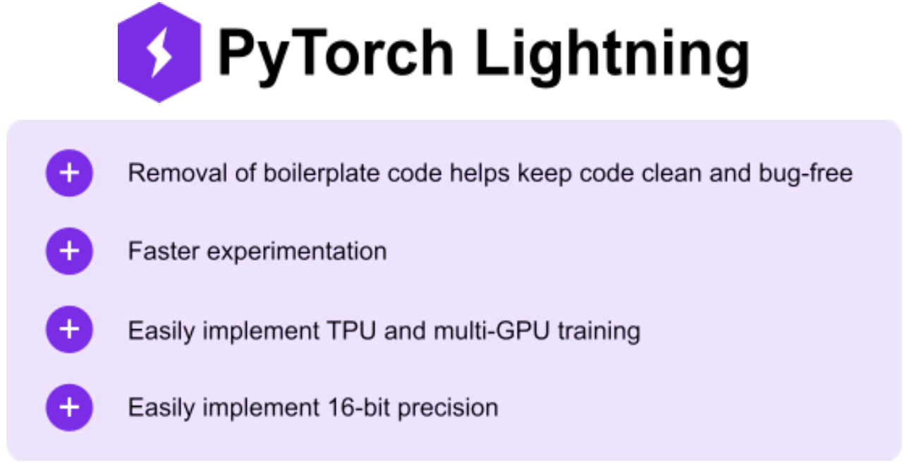
Enter: PyTorch Lightning. Lightning is a high-level framework for PyTorch that abstracts away implementation details so you can focus on building great models and forget about wasting time on trivial details. Benefits abound:
How to Install PyTorch Lightning
First, we’ll need to install Lightning. Open a command prompt or terminal and, if desired, activate a virtualenv/conda environment. Install PyTorch with one of the following commands:
pip
conda
Lightning vs. Vanilla
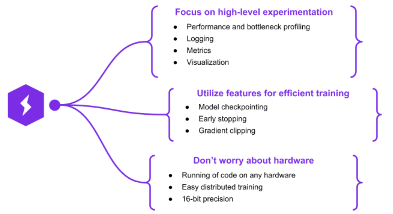
PyTorch Lightning is built on top of ordinary (vanilla) PyTorch. The purpose of Lightning is to provide a research framework that allows for fast experimentation and scalability, which it achieves via an OOP approach that removes boilerplate and hardware-reference code. This approach yields a litany of benefits.
PyTorch Lightning Workflow
One of the greatest benefits of Lightning is its ease of use, which stems from the fact that it is, in essence, a hardware-agnostic wrapper for boilerplate PyTorch. What this means in practice is that the code is exactly the same as vanilla PyTorch, but it is cast in a convenient object-oriented way that allows users to focus on the important components of the training process. Much of this difference is encapsulated in and highlighted by the difference between a PyTorch Model and a Lightning Module.
PyTorch Modules
The PyTorch nn.Module class is the base class for neural networks in PyTorch from which all designs are subclassed. While it is possible for a module to contain other modules in a nested fashion, this is usually not done.
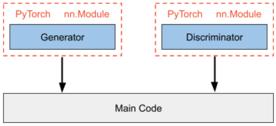
Consider the case of training a Generative Adversarial Network (GAN). In such a network, a generator creates fabricated data that is intended to mimic a set of real data, and a discriminator seeks to differentiate between the real and fabricated data.
In vanilla PyTorch, the typical way of defining and training such a system would be to create generator and discriminator classes by subclassing the nn.Module, and then instantiating and calling them in the main code, in which you have manually defined forward passes, loss calculations, backwards passes, and optimizer steps.
Lightning Modules
In contrast, a LightningModule defines an entire deep learning ecosystem. Continuing with the example of training a GAN, we have generator and discriminator models, loss functions, training/testing/validation functions, and optimizers. This entire system is encapsulated by the Lightning Module.
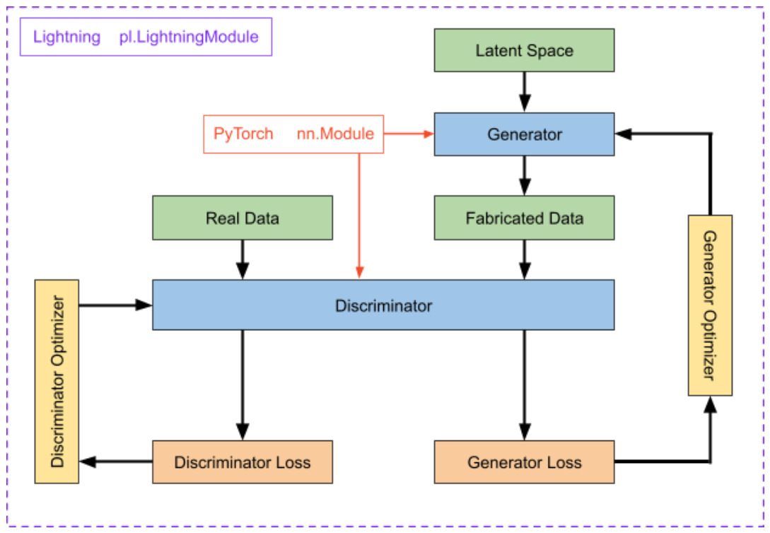
It is important to note that a LightningModule does not build abstractions on top of vanilla PyTorch code, but simply organizes it in a more efficient and cleaner manner.
Lightning Module Components
A lightning module is composed of six components which fully define the system:
- The model or system of models
- The optimizer(s)
- The train loop
- The validation loop
- The test loop
- The prediction loop
Only the essential features of each of these components is defined in its respective class/function. This removal of boilerplate permits cleaner code and lowered probability of making a trivial error; however, any part of training (such as the backward pass) can be overridden to maintain flexibility.
Now that we have a better picture of Lightning workflow, let’s dive into an example that highlights the power and simplicity of Lightning!
Building a GAN with PyTorch Lightning
We’ll construct a GAN using Lightning and compare it to vanilla PyTorch afterwards, highlighting the places in which Lightning made our lives easier. First, a recap of GANs (or an introduction for the uninitiated).
Generative Adversarial Networks
Deep Learning is an indispensable tool for a wide variety of tasks. At AssemblyAI we utilize its power for features such as Entity Detection, Sentiment Analysis, Emotion Detection, Translation, and Summarization. Many of the tasks that Deep Learning is adept at involve processing data to extract some useful information, but what if we want instead to generate data?
GANs allow for the generation of data (hence “generative”) by learning a distribution which mirrors that of a specific set of input data. Once the distribution is learned, data can be generated that is similar but distinct from the input data, so much so that it can become impossible for humans to perceive a difference. Can you tell which celebrity pictures below are fabricated?

If you guessed “all of them”, you’d be correct!
The power of GANs stems from the fact that two Deep Learning models, the generator and the discriminator, are pitted against one another in a zero-sum game (hence “adversarial”'). As the generator gets better at fabricating more convincing data, the discriminator learns to become better at differentiation; as the discriminator becomes more discerning in its detection of fabricated data, the generator learns to produce more convincing forgeries.
GAN for Handwritten Digits in Lightning
We’ll use the canonical MNIST dataset to construct a GAN in Lightning that is capable of reproducing handwritten digits. First, we need to download and process this data. Lightning again provides a structured framework for this procedure in the form of LightningDataModules.
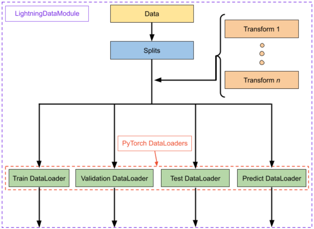
Lightning DataModule
A LightningDataModule is simply a collection of PyTorch DataLoaders with the corresponding transforms and downloading/processing steps required to prepare the data in a reproducible fashion. It encapsulates all steps requires to process data in PyTorch:
- Download and tokenize
- Clean and save to disk
- Load inside Dataset
- Apply transforms
- Wrap inside a DataLoader
Importantly, a LightningDataModule is shareable and reusable. That is, it centralizes all data preparation tasks to have a self-contained object that can exactly duplicate a dataset via identical splits and transforms.
Let’s create our MNIST LightningDataModule. First, we initialize with some relevant parameters and create the transform object that we will use to process our raw data. Lastly, we create a dictionary which we will pass into our DataLoaders later.
Next, we define the prepare_data() function. It defines how to download and e.g. tokenize data. Lightning ensures that this method is called with a single process to avoid corrupted data. Here, we simply download our training and testing sets.
Next up is the setup() function. It defines data operations you might want to perform on every GPU. Use it to define datasets and e.g. split/transform data or build a vocabulary. In our case, we will split the data into training, validation, and testing sets, using our transform defined in the class __init__() function.
Finally, we define training, validation, test, and predict DataLoaders. Usually the datasets defined in setup() are simply wrapped in DataLoader objects. Note that validation data is not really necessary for GANs given their unusual evaluation protocols, but nevertheless val_dataloader() is added here for completeness. Further, we have not defined a predict DataLoader here, but the process is identical.
Building the Lightning Module
Recall from above that the central object in the Lightning workflow is the LightningModule, which encapsulates the entire model ecosystem. Now that we’ve finished defining our LightningDataModule object, we can build our LightningModule. In our case, this ecosystem includes two models - the generator and the discriminator. We’ll define them now, noting that the process is identical to vanilla PyTorch.
Building the Discriminator
First, we’ll construct our discriminator as an nn.Module. We’ll use a simple CNN with two convolutional layers followed by a fully connected network to map from 28x28 single channel digit images to classification predictions. Remember, the purpose of the discriminator is to classify images as real or fake, so we only need a single output node, in contrast to the ten required for the digit classification networks often built for MNIST.
Next, we define the forward pass for the discriminator. We use max poolings with a kernel size of two followed by ReLU for the convolutional layers, and use sigmoid for the final activation
Building the Generator
Similarly, we construct the generator as an nn.Module. We input data points from a latent space which feed into a linear layer to provide us with enough nodes to create 7x7 images with 64 feature maps. We then used transposed convolutions for learnable upsampling, ultimately collapsing the data to a 28x28 single channel image (i.e. the digit image) via a final convolutional layer.
And again, we define the forward pass.
Defining the GAN
Now that we have our traditional PyTorch nn.Module models, we can build our LightningModule. This is where we will see the Lightning approach diverge from the vanilla PyTorch approach.
Initialization
First, we define our initialization function, inputting our latent dimensionality as well as a learning rate and betas for our Adam optimizers. save_parameters() allows us to store these arguments under the self.hparams attribute (also stored in the model checkpoint) for easier reinstantiation after training. Finally, we initialize the generator and discriminator models within our ecosystem, and generate latent space points that we can use to monitor progress. These points will give us a consistent set of data to track how the generator is progressing in mapping from the same set of latent points to images as it learns.
Forward Pass and Loss Function
Next, we define the GAN’s forward pass and loss function. Note that using self.generator(z) is preferred over self.generator.forward(z) given that the forward pass is only one component of the calling logic when self.generator(z) is called.
We will be using the loss function in two different ways - one as the discriminator loss and one as the generator loss. The first way is to update the discriminator as a classifier in the canonical fashion, inputting real and generated images with the appropriate labels. The second way is to update the generator using the loss from the discriminator on generated images. That is, the better the discriminator is at detecting fake images, the more the generator is updated. More on this later.
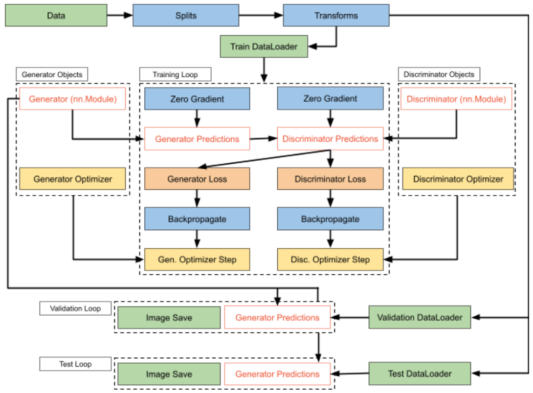
Training Step
Next up is defining what occurs during a training step for the GAN. If we are training the generator, we generate images and then get predictions on them via the discriminator. When we calculate the loss, we are importantly using deceptive labels here. That is, despite the fact that the images are fabricated, we label them as real in the loss function. This is because we want them to be classified as real, so the deceptive labels will lead to greater loss when the generated images are (correctly) classified as fake. We also log some of the fabricated images to be viewed in TensorBoard, and output relevant values.
There are no special details for training the discriminator. In a very straightforward fashion, we compute the loss on the real images and the fake images (with honest labels) and average them as the discriminator loss. Again we output the relevant parameters.
Configure Optimizers
Now we can configure our Adam optimizers using the learning rates and betas we saved in self.hparams. We configure one optimizer for the generator and one for the discriminator.
Epoch End
Finally, we define the on_epoch_end() method. It is not strictly necessary, but we use it here to log images so that we can observe training progress across epochs. It is called whenever a training, testing, or validation epoch ends. Note that each of the training, testing, validation, and predict cases have their own epoch_end() functions in case you do not want to perform such a function across the board!
Program Code
Now we can write the main program code to utilize all of the components we’ve defined above, which requires just a few simple lines with Lightning.
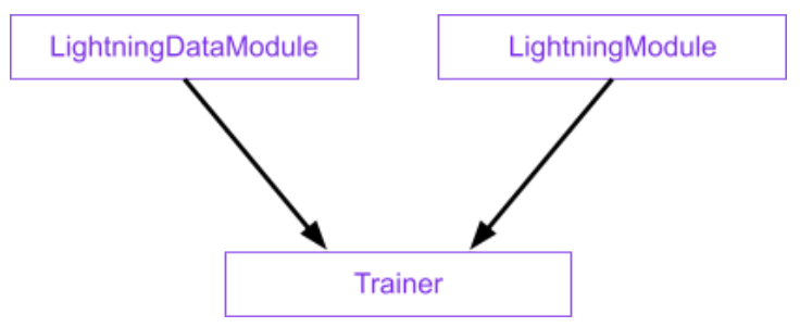
Lightning Trainer
Recall from above that the LightningModule is not an abstraction layer on top of PyTorch, but simply a reorganization of code. The abstraction in Lightning comes from the Trainer class. The Trainer class has very straightforward minimal usage, and is the source of many benefits, including:
- The ability to override any automation component
- The omission of hardware references
- The removal of boilerplate code
- The inclusion of under-the-hood best practices via contributors from top AI labs
For our purposes, we simply need to pass in a value for the maximum number of training epochs.
GAN Training
We’ve defined our LightningDataModule and LightningModule above and instantiated the trainer which will operate on our LightningModule. Now all we need to do is instantiate our LightningDataModule and LightningModule and pass them in to the trainer!
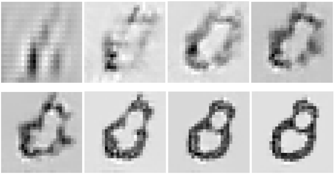
Results
Recall that we were using the same latent space points as validation throughout training. That means we can compare how the same point was mapped from latent space to a digit image throughout training. Below we’ve selected one such point and displayed the output images from passing it through the generator as training progressed. Pretty good results!
PyTorch Lightning vs Vanilla
For users experienced with vanilla PyTorch, the benefits of Lightning are sure to make themselves evident. Lightning offers the ease of automation with the flexibility of overriding, utilizing convenient classes that ensure reproducibility. In addition, a lack of hardware references and the omission of manual backpropagations and optimizer steps make distributed training a breeze.
In our GAN example, many of these differences are readily apparent. After defining out (reusable and shareable) LightningDataModule object and encapsulating our training ecosystem in a LightningModule, our main code looks like this:
On the other hand, training a GAN even as simple as the one laid out above looks like this:
It is easy to see how such a workflow is not scalable to more complicated Deep Learning ecosystems.
Final Words
PyTorch Lightning provides a powerful and flexible framework for experimenting and engineering scalable models for deep learning. We have seen how its object-oriented approach compartmentalizes code into efficient components and avoids training code that is messy or scattered across many different files. The minimum usage of PyTorch is very straightforward, and the ability to override automated processes allow users to maintain control as models get more complex.