

At the bedrock of the Deep Learning that powers incredible technologies like text-to-image models lies matrix multiplication. Regardless of the specific architecture employed, (nearly) every Neural Network relies on efficient matrix multiplication to learn and infer. Finding efficient and fast matrix multiplication algorithms is therefore paramount given that they will supercharge every neural network, potentially allowing us to run models prohibited by our current hardware limitations.
Recently, DeepMind devised a method to automatically discover new faster matrix multiplication algorithms. The method employs AlphaTensor, an AI-based system that operates on Deep Reinforcement Learning.
In this article, we will highlight AlphaTensor’s major impacts and learn how it works under-the-hood.
Introduction
The discovery of faster matrix multiplication algorithms has far-reaching implications. Even beyond the specific context of Neural Networks, matrix multiplication lies at the foundation of much of modern computing, playing a fundamental role in computer graphics, digital communications, and scientific computation. Each of these fields could benefit significantly from new, more efficient algorithms.
AlphaTensor is a system able to autonomously search for provably correct matrix multiplication algorithms. Among its achievements, here are some highlights:
- AlphaTensor automatically rediscovered the current State-of-the-Art matrix multiplication algorithms and improved on the best know complexity in several cases.
- AlphaTensor can be trained to search for efficient algorithms tailored to specific hardware without any prior knowledge.
- AlphaTensor takes advantage of the tools AlphaZero used to play Chess and Go to explore the (gigantic) search space of potential algorithms. From a mathematical standpoint, the large amount of valid new algorithms discovered by AlphaTensor imply that this space is richer than previously known. This represents a novel approach to searching large combinatorial spaces of this nature.
While these results are impressive, the improvements of the new algorithms discovered by AlphaTensor do not represent a major breakthrough for the general problem of the complexity of matrix multiplication, which we will discuss later. The most exciting part about AlphaTensor lies not in its results, but in the novel ideas it introduces, and the potential for further extensions.
A potential blueprint for algorithm discovery
The potential applications of AlphaTensor are not necessarily limited to the specifics of matrix multiplication. The system’s underlying design is a general purpose architecture and, thanks to its flexibility, it could be adapted to search for other types of algorithms that optimize a variety of distinct metrics.
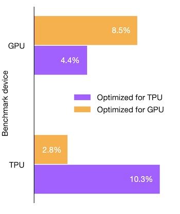
Examples of such metrics are: speed, memory, numerical stability, energy usage, or even the adaptability of a given algorithm to a specific target hardware. The last one, in particular, is implemented in the paper to optimize one case of matrix multiplication for the Nvidia V100 GPU, and Google's TPU v2. The results are shown in the following chart:
AlphaTensor's point of departure is a reformulation of matrix multiplication in the language of tensors (we explain how this works and what tensors are in the sections below). Because tensors can represent any bilinear operation, such as structured matrix multiplication, polynomial multiplication, or more custom bilinear operations used in specific areas of computing, further extensions of AlphaTensor targeting other mathematical problems could unlock new possibilities for research in complexity theory and other areas of mathematics.
How does AlphaTensor search for new algorithms?
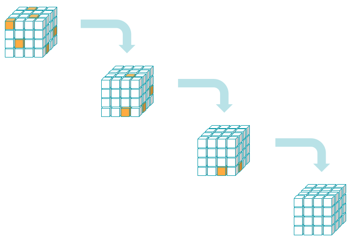
For now, let us just picture tensors as a sort of abstract analogue of a Rubik's cube, like in the figure below:
AlphaTensor is able to self-learn how to play a single-player game called TensorGame, where the player manipulates a given input tensor in a way that results in a set of instructions representing a new multiplication algorithm.
TensorGame is played by utilizing and improving upon the techniques developed to self-learn board games like Chess or Go, famously solved by DeepMind’s AlphaZero model. Note that the number of degrees of freedom for TensorGame, i.e. the amount of possible actions a player can take at every move, is several orders of magnitude higher than in Chess or Go, which makes this problem extremely difficult. More details on TensorGame in a section below.
A high-level overview of how AlphaTensor operates will be given below, followed by some expanded details of its individual components.
Before that, let us first give an answer to the following natural questions:
- Can matrix multiplication be improved at all?
- What is a tensor? And in which sense a tensor decomposition is equivalent to a matrix multiplication algorithm?
Why matrix multiplication is not optimal
The standard way to multiply two matrices is not a very efficient algorithm. The reason is simple: for a computer, multiplication (of two numbers) is a more computationally expensive (slower) operation than addition. This is because addition of two numbers in binary form works in parallel –with only one cycle over the bits– whereas multiplication implies a series of additions and bit-shifting operations, hence several cycles.
Therefore, reducing the total number of multiplications required for any computational task (even at the cost of incrementing the number of additions/subtractions), effectively speeds up the whole process and yields a faster implementation.
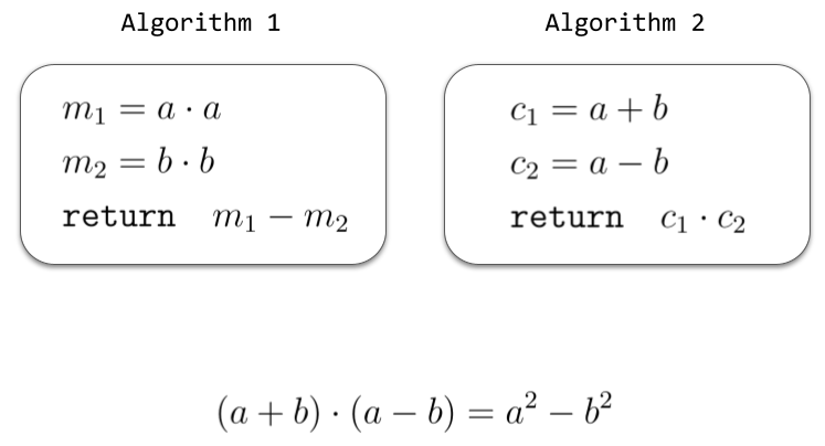
A simple example: two different algorithms for computing the difference of the squares of two numbers \(a\) and \(b\) are shown in the figure below. Both algorithms return the same result, but the second one is more efficient, requiring half as many multiplications as the first one.
How many multiplications are required to multiply two matrices? This depends both on the size of the matrices as well as on the chosen implementation. For two matrices of size \(2 \times 2\), the standard algorithm requires 8 multiplications, as illustrated in the next figure.
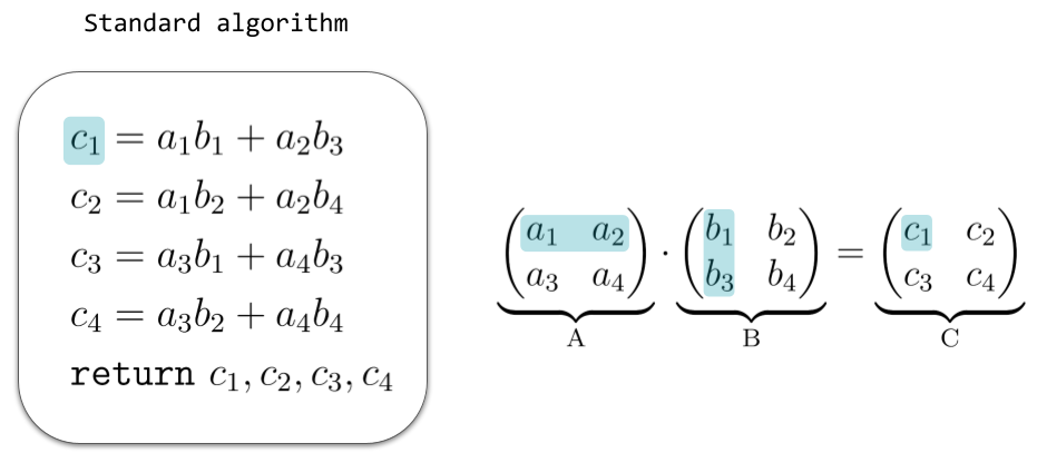
More generally, in order to multiply two (compatible) matrices \(A\) and \(B\) with the standard algorithm, one has to multiply each row of \(A\) with each column of \(B\) and each such operation requires \(n\) multiplications, where \(n\) is the length of a row vector of \(A\). Thus, in total we need:\[ ( \text{num. of rows of } A) \times ( \text{num. of columns of } B) \times (\text{num. of columns of } A) \text{ multiplications} \] In the case of square matrices of size \(n \times n\) this becomes \(n^3\), so one says that the standard algorithm has a cubic complexity in the input matrix size, written \( O(n^{3}) \).
Is it possible at all to come up with a faster algorithm for matrix multiplication?
The answer is yes, and goes back to an important discovery from 1969, by the German mathematician Volker Strassen. He was the first one to realize that the standard algorithm was not optimal, and discovered an algorithm that requires only \(7\) multiplications for the \(2 \times 2\) case.
While Strassen’s discovery is extremely important, it doesn’t offer any systematic method for searching for new matrix multiplication algorithms. Testing all possible combinations is not feasible in practice, even for a brute-force computer program running on the fastest available machine, as the number of such combinations is completely out of reach, already for low-size matrices. The number of admissible algorithms in the \(4 \times 4\) case for example, already increases by \(10^{10}\) times over the \(3 \times 3\) case.
Then, how do we go about systematically searching for new multiplication algorithms? A very smart thing to do, it turns out, is to reformulate the problem in a different context: that of tensor decompositions.
Tensors as higher-dimensional matrices
A tensor is a generalization of the notion of matrix. If we think of a matrix \(A\) as given by a list of numbers

indexed by two indices \(i\) and \(j\) (each running in a given range), a 3D-tensor \( \mathcal{T} \) is given by a list of numbers

indexed by three indices \(i,j,k\). Adding even more indices, this quickly generalizes to the notion of 4D, 5D, or even higher-dimensional tensors. In this way, we see how matrices are in fact just a special example of tensors: matrices are 2D-tensors.
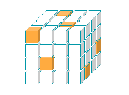
Just like a matrix (or 2D-tensor) can be visualized as a "square-table" (or more generally a rectangle-table) of numbers, it is natural to visualize a 3D-tensor as a 3D-box of numbers. If, moreover, a tensor's only possible entries are 0 and 1, we can just use coloured boxes to represent a value of 1, with the remaining ones being zero, as in the following image:
A matrix multiplication algorithm is a tensor decomposition
The starting point is the following observation: once the matrix sizes are fixed, there is a unique 3D-tensor \(\mathcal{T}\) (containing only 0 and 1) that represents the multiplication \(AB = C\) of any pair of matrices \(A\) and \(B\) of the given size. More is true: any decomposition of \(\mathcal{T}\) (see the example below) will automatically yield a new set of instructions for how to do this multiplication, i.e. to a specific multiplication algorithm. The upshot is: finding new matrix multiplication algorithms is equivalent to finding decompositions of the corresponding tensor.
To explain how this works, let us illustrate the \(2 \times 2\) case:
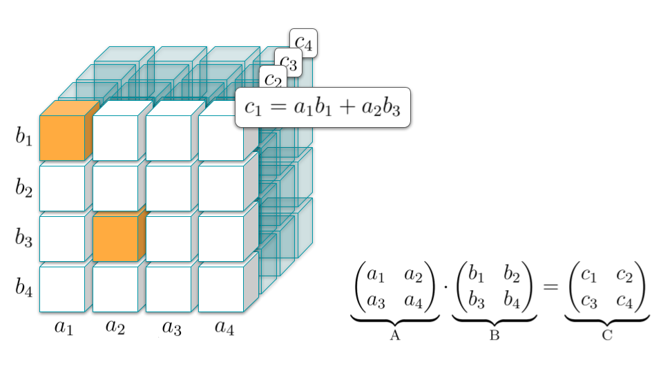
The figure shows the tensor \(\mathcal{T}\) representing matrix multiplication in the \(2 \times 2\) case. The first slice of \(\mathcal{T}\) (highlighted in the front) contains the recipe for expressing the first coefficient \(c_1\) of the matrix \(C\) in terms of the coefficients of \(A\) and \(B\). Similarly, the other slices do the same for the remaining coefficients of \(C\).
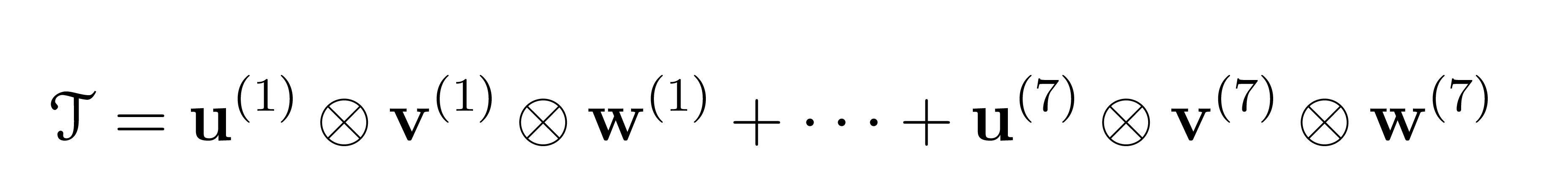
Once the size of \(A\) and \(B\) is fixed, the construction of the tensor \(\mathcal{T}\) is a straightforward operation. The crucial point now is that \(\mathcal{T}\) can admit several distinct decompositions in terms of sums of outer products of three vectors, i.e. of the following form:

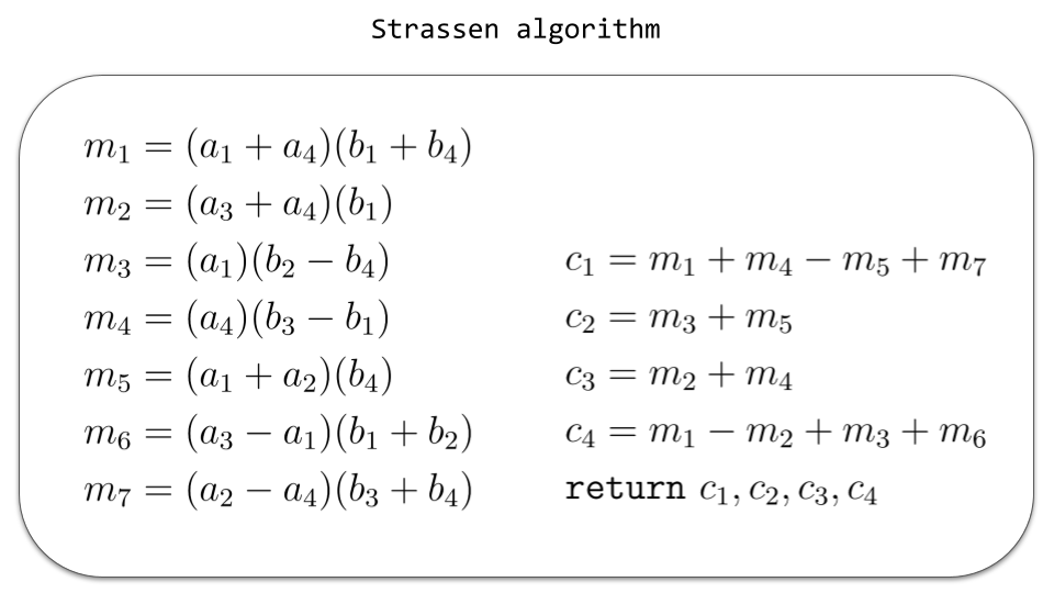
Each individual factor \(\mathbf{u} \otimes \mathbf{v} \otimes \mathbf{w} \) amounts to one multiplication step in the algorithm corresponding to such a decomposition. The next figure illustrates how this mechanism works in the case of Strassen’s algorithm:

To sum up, in order to find a new algorithm (with exactly \(R\) multiplications) it is enough to find a decomposition of the tensor \(\mathcal{T}\) as a sum of exactly \(R\) products \(\mathbf{u} \otimes \mathbf{v} \otimes \mathbf{w} \) as above. The problem is that the number of all such decompositions is enormous – in fact, just as big as the number of matrix multiplication algorithms. Some sophisticated strategies are needed in order to explore this combinatorial space. The way AlphaTensor does it is by playing a 3-dimensional board game, named TensorGame.
TensorGame
Tensor decomposition can be rephrased as a reinforcement learning problem, modelling the environment as a single-player 3D board game, TensorGame.
Goal of the game: given any tensor \(\mathcal{T}\), we want to find a decomposition of \(\mathcal{T}\) as a sum of \(R\) outer products (as in the previous section) with \(R\), which corresponds to the number of multiplications in the algorithm, as small as possible.
The game is played as follows:
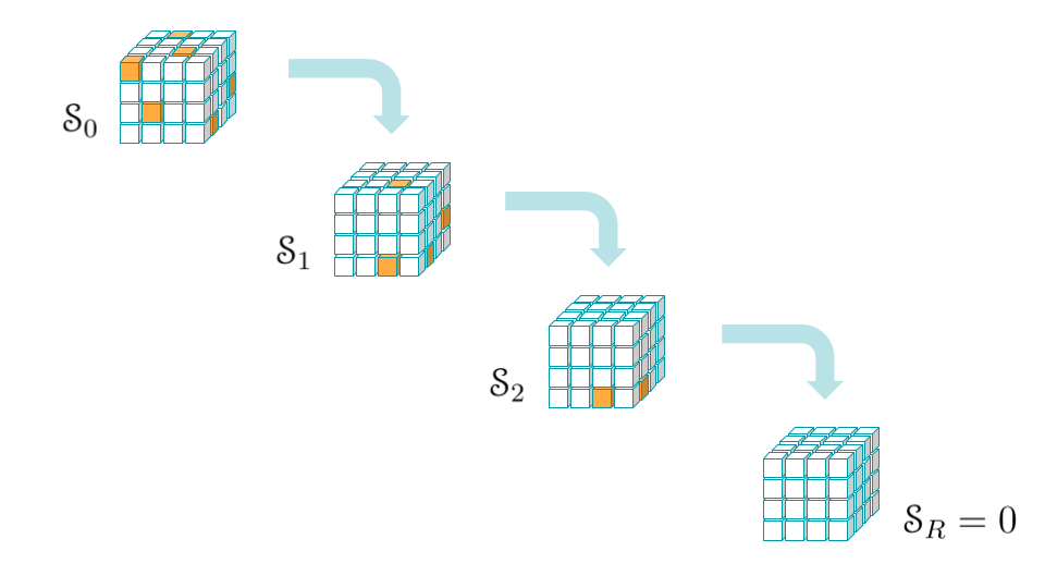
- Step zero (t = 0): The initial state is set to be the target tensor we want to decompose:

- Step t (t = 1,2,3,...): the player selects three vectors:

and the new state is updated recursively to:

- End of the game: after R steps, the player reaches the zero-tensor:
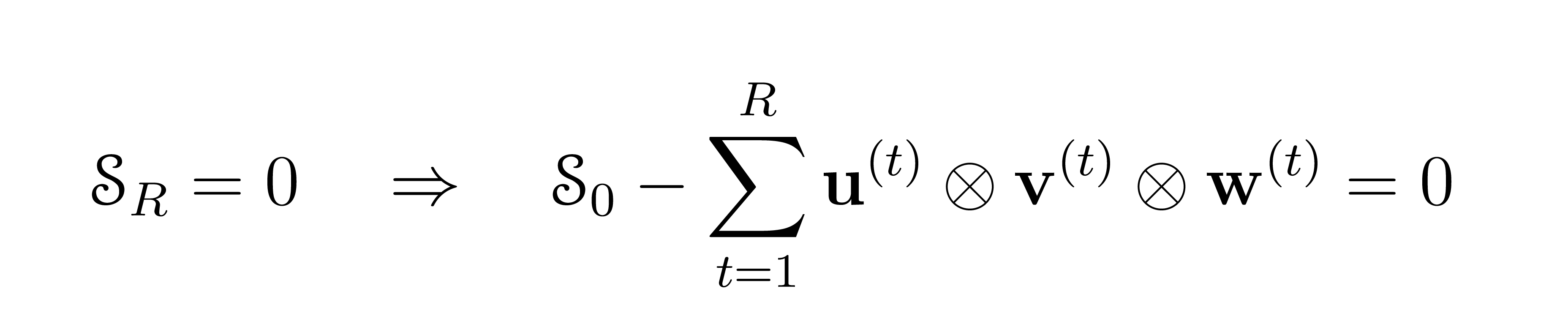
in which case this yields a tensor decomposition of the initial tensor \(\mathcal{T}\). At each step \(t\) there is a negative reward, encouraging fewer steps to reach zero. Only a preset maximum number of moves is allowed: an additional negative reward is applied in the event the player terminates with a non-zero vector after this limit.
AlphaTensor - Overview of the model
AlphaTensor is built around a Deep Reinforcement Learning paradigm: an agent is able to search the space of tensor decompositions by playing TensorGame. The actions are taken using a policy and reward functions and played games are fed into a neural network that updates and improves policy and reward. More specifically, the whole process consists of the following steps:
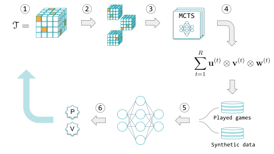
- TensorGame begins: Input a 3D tensor \( \mathcal{T}\) corresponding to the multiplication \(AB = C\).
- Data augmentation step: \(\mathcal{T}\) is transformed by a random sample of base-changes (these are equivalent ways to represent the same tensor according to different reference systems). AlphaTensor is forced to play the game in all bases in parallel. The key point is that it is sufficient to find a decomposition in any of the bases. This also automatically injects diversity into the games played.
- Series of Monte Carlo tree search (MCTS) steps combined with reinforcement learning to decide on next action, until the end of the episode. MCTS operates guided by a policy function and a value function. The policy function is used to decide which steps to take to go down the tree. The value function is used to estimate the reward of the chosen path.
- The output is a played game, equivalent to a decomposition of \(\mathcal{T}\), and is added to a list of played games.
- Deep Reinforcement Learning begins: Sample a state randomly from either the list of played games or a prepared list of synthetic data and feed this to a neural network, trained to learn and update the policy and value functions used in the MCTS.
- The model is updated with the new policy and value functions. A new iteration can start.
These points represent a schematic overview of the main components of the AlphaTensor model in action. Let's take a closer look at some of these components.
Data augmentation strategies
AlphaTensor uses some interesting data augmentation strategies, taking advantage of various symmetries of the problem as well as applying tricks from linear algebra.
At the start of each game episode, the input tensor is augmented by applying a sample of base-changes, as mentioned in the above overview. Specifically, a change of basis is determined by a (sampled) choice of three invertible matrices which are applied to the original tensor. If the player finds a tensor decomposition of any of the transformed tensors, it is straightforward to convert such decomposition into a decomposition in the original (canonical) basis. The rank \(R\) of the decomposition is preserved in this process. In practice, the number of these randomly generated bases is around 100,000, and AlphaTensor plays games in all bases in parallel.
Another strategy involves a prepared list of synthetic data. Although tensor decomposition is a NP-hard problem, the inverse task of constructing the tensor from its factors is elementary. A synthetic dataset of tensor factorizations is thus easily generated by taking random samples of vector triples \(\mathbf{u}^{(t)}, \mathbf{v}^{(t)}, \mathbf{w}^{(t)}\), for \(t=1, \dots, R\) and then adding their products together to construct a random tensor \(\mathcal{T}\). This yields a large list of tensor-factorization pairs that can be used for supervised learning. In fact, AlphaTensor's neural network employs a mixed training strategy: training at once on the target tensor with a standard reinforcement learning loss and on random tensors with a supervised loss.
From every played game, an additional tensor-factorization pair is extracted by swapping a random action with the last action, exploiting the commutativity of the addition in the tensor factorization. This yields an additional pair for supervised learning at each iteration.
Sample-based Monte Carlo tree search (MCTS) in action
When playing TensorGame, at each move one can assign a search tree of possibilities. Specifically, the search consists of a series of simulated trajectories of TensorGame that are aggregated in a tree. The search tree therefore consists of nodes representing states \( (\mathcal{S}_t) \) and edges representing actions. One action corresponds to the choice of three vectors \(\mathbf{u}, \mathbf{v}, \mathbf{w}\), which results in a huge number of possibilities at each level of the tree.
Instead of traversing the whole tree and visiting every node, MCTS samples a subset of the tree. The actions are sampled based on the policy function, and the action with the highest potential reward is selected. The value function is used for evaluating a given sequence of actions, i.e. a given trajectory down the tree.
A transformer-based neural network architecture
AlphaTensor uses a deep neural network to guide the Monte Carlo tree search. Let us highlight the main features of its architecture.
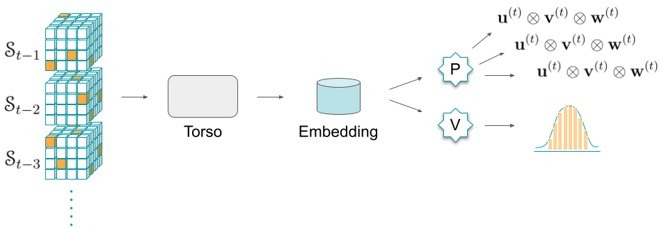
The neural network is composed of a common torso (acting as an encoder), followed by a double head. More specifically:
- The input is the current state, together with a history of previous states.
- The torso is based on a modification of transformers which utilizes a special form of attention mechanism called axial attention. Its purpose is to create a representational embedding of the input that is useful for both policy and value heads.
- The policy head's purpose is to predict a distribution over potential actions. It uses a transformers architecture to model an autoregressive policy. Autoregressive here means that the model acts by measuring the correlation between observations at previous time steps to predict the output (similar to a decoder architecture in language models).
- The value head is composed of a multilayer perceptron and trained to predict a distribution of the returns from the current state (cumulative reward).
A review of AlphaTensor's results
For matrices of small size, a comparison between the complexity of previously known matrix multiplication algorithms and the ones discovered by AlphaTensor is shown in the following table:
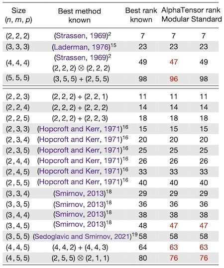
The first column shows the size of the matrices considered: for example (4,4,5) refers to the problem of multiplying a 4 x 4 matrix with a 4 x 5 matrix. The word rank here refers to the total number of scalar multiplications used in the algorithm. This is the way the complexity is measured. The last two columns show the rank obtained by AlphaTensor in modular arithmetic (specifically: modulo two) and standard arithmetic respectively.
For the cases of square matrices considered (first rows in the table) AlphaTensor improves on the best known rank only for modular arithmetic. There are also 3 improvements in the non-square cases that hold for real matrices. In a second table (see Extended Data Table 1 in the original paper) the authors are able to combine some of the low-size algorithms and get improvements over the best known rank for several cases, in size up to (11,12,12).
It is remarkable to note that AlphaTensor automatically rediscovers the current State-of-the-Art algorithm in each of the cases considered. On the other hand, while these results are impressive, the improvements do not represent a major breakthrough for the problem of matrix multiplication.
The speedups reported in the paper are mostly between 1% and 6% for standard arithmetic and seem to have been measured only on synthetic data. Presumably, the algorithms have been tested on randomly generated matrices, although this is not specified by the authors. Describing explicitly the structure of the test set should be established best-practice in machine learning research papers, to avoid any risks related to data leakage and ensure reproducibility of the results.
It is also worth to note that the matrices appearing in real-world applications often come with very special structure, and the improvements of the new algorithms on this kind of data have yet to be demonstrated. For example, it would be extremely interesting to test the new algorithms on sparse matrices (which are ubiquitous in applications) or more generally analyzing actual case-studies such as computer graphics, scientific simulation or the training of neural networks. Unfortunately, the authors do not report any test done in these settings.
While the algorithms can be applied recursively to matrices of higher size (for example, the 4 x 4 algorithm can be applied to any square matrix with size equal to powers of 4) and there the advantages become apparent, this typically means astronomically large matrices, rarely seen in real-world applications.
On a different note, it might be worth to remark that speed is often not the paramount feature for practical uses of matrix multiplication. Numerical stability is arguably of utmost importance in many computational tasks. Although AlphaTensor can be set to target such a metric, there are no experiments in this direction appearing in the paper, and the numerical error bounds of the newly discovered algorithms are not reported.
Final words
Matrix multiplication is a fundamental operation in linear algebra. It forms the basis for many other matrix operations and is widely used, for example, in applied mathematics, computer science and several areas of engineering and scientific computation. Both the theoretical understanding of the complexity of matrix multiplication and the development of fast practical algorithms are of great interest.
AlphaTensor is an AI system based on Deep Reinforcement Learning that can independently find novel and provably correct algorithms for complex mathematical tasks. Trained to specifically attack the problem of matrix multiplication, it has already shown very interesting results, and its potential for further extensions and applications to other tasks in automatic algorithm design appears to be promising.