How Imagen Actually Works

While the Machine Learning world was still coming to terms with the impressive results of DALL-E 2, released earlier this year, Google upped the ante by releasing its own text-to-image model Imagen, which appears to push the boundaries of caption-conditional image generation even further.

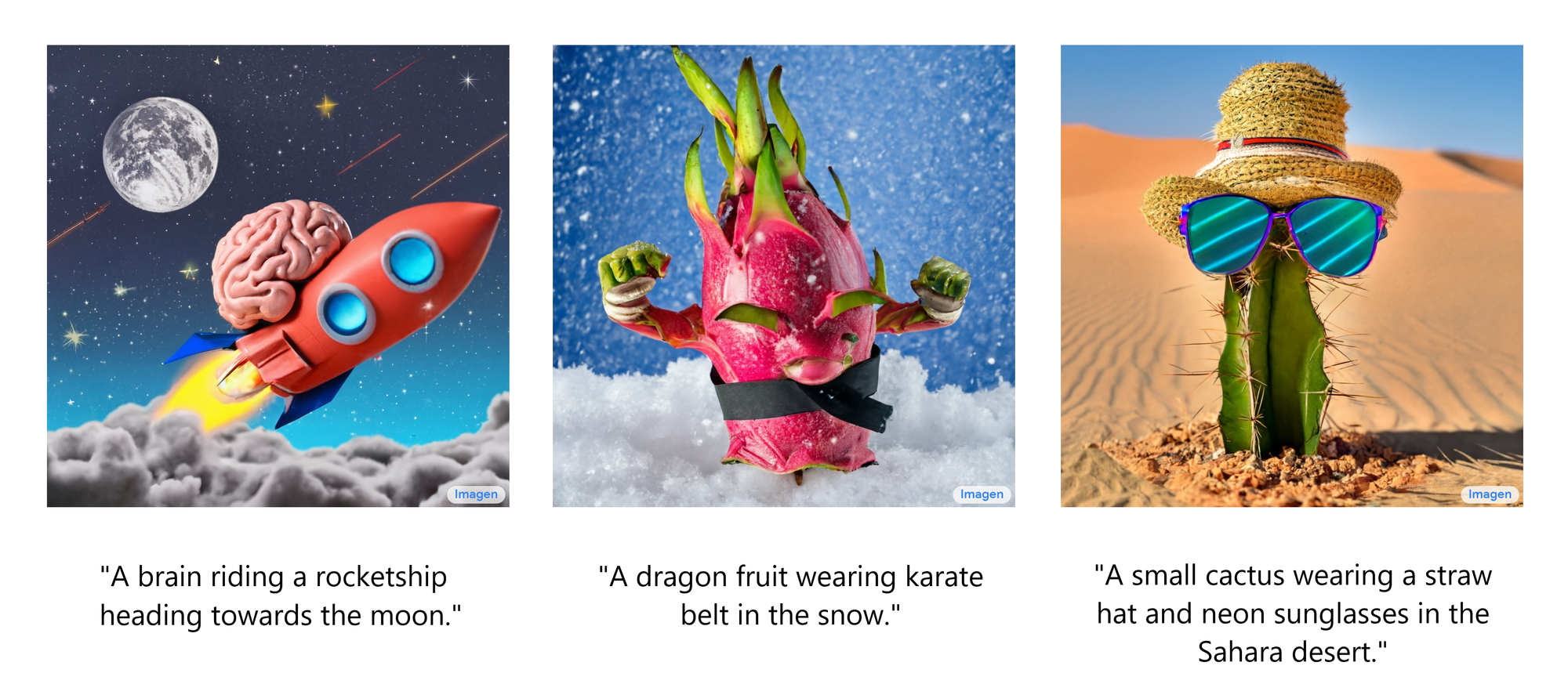
Imagen, released just last month, can generate high-quality, high-resolution images given only a description of a scene, regardless of how logical or plausible such a scene may be in the real world. Below you can see several examples of such images with their corresponding captions beneath:

These impressive results no doubt have many wondering how Imagen actually works. In this article, we'll explain how Imagen works at several levels.

First, we will examine Imagen from a bird's-eye view in order to understand its high-level components and how they relate to one another. We'll then go into a bit more detail regarding these components, each with its own subsection, in order to understand how they themselves work. Finally, we'll perform a Deep Dive into Imagen that is intended for Machine Learning researchers, students, and practitioners.

Without further ado, let’s dive in!

Introduction

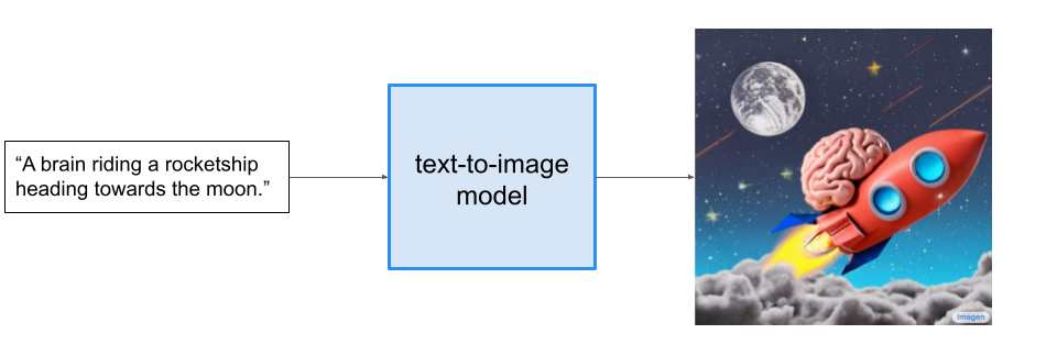
In the past few years, there has been a significant amount of progress made in the text-to-image domain of Machine Learning. A text-to-image model takes in a short textual description of a scene and then generates an image which reflects the described scene. An example input description (or "caption") and output image can be seen below:

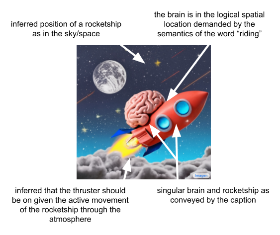
It is important to note that high-performing text-to-image models will necessarily be able to combine unrelated concepts and objects in semantically plausible ways. These models must therefore overcome challenges like capturing spatial relationships, understanding cardinality, and properly interpreting how words in the description relate to one another. If we more closely inspect the image from the above figure, we can see that Imagen performs well on these fronts upon first inspection.

It is hard to overstate just how impressive these models are. They are not using a database to search for and return an image which matches the description, and they are not even "stitching" together pre-existing sub-images in a clean way such that the result corresponds to the caption. They instead generate entirely novel images that convey visually the semantic information contained in the caption.

Now that we understand what text-to-image models are in general, we can take a look at how the text-to-image model Imagen works from a bird's-eye view.

How Imagen Works: A Bird's-Eye View

In this section, we'll learn what the salient components of Imagen do and how they relate to one another. First, we'll look at the overarching architecture of Imagen with a high-level explanation of how it works, and then inspect each component more thoroughly in the subsections below.

Here is a short video outlining how Imagen works, with a breakdown of what's going on below:

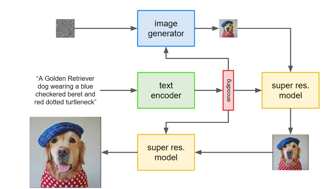
1. First, the caption is input into a text encoder. This encoder converts the textual caption to a numerical representation that encapsulates the semantic information within the text.
2. Next, an image-generation model creates an image by starting with noise, or "TV static", and slowly transforming it into an output image. To guide this process, the image-generation model receives the text encoding as an input, which has the effect of telling the model what is in the caption so it can create a corresponding image. The output is a small image that reflects visually the caption we input to the text encoder.
3. The small image is then passed into a super-resolution model, which grows the image to a higher resolution. This model also takes the text encoding as input, which helps the model decide how to behave as it "fills in the gaps" of missing information that necessarily arise from quadrupling the size of our image. The result is a medium sized image of what we want.
4. Finally, this medium sized image is then passed into yet another super-resolution model, which operates near-identically to the previous one, except this time it takes our medium sized image and grows it to a high-resolution image. The result is 1024 x 1024 pixel image that visually reflects the semantics within our caption.

At the highest level, that is all there is to it! For a slightly more detailed look at each of Imagen's big components, check out the below subsections. Otherwise, you can jump down to the Deep Dive section to get into the nitty-gritty of how Imagen works, or jump straight down to the Final Words.

Text Encoder

In this subsection, we will take a closer look at Imagen's text encoder. As we can tell from the above video, the text encoder is critical to Imagen's performance. It conditions all of Imagen's other components and is responsible for encoding the textual caption in a useful way.

The text encoder in Imagen is a Transformer encoder. If you are unfamiliar with Transformers, don't worry. The most important detail here is that such an encoder ensures that the text encoding understands how the words within the caption relate to one another (by a method called "self-attention"). This is very important because the English language encodes information via its syntactic structure that affects the semantic meaning of a given sentence.

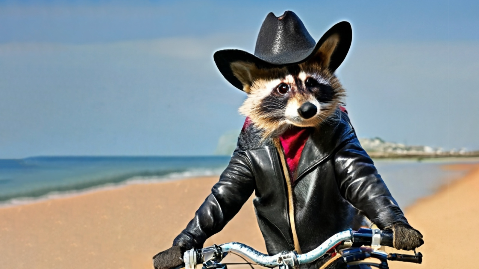
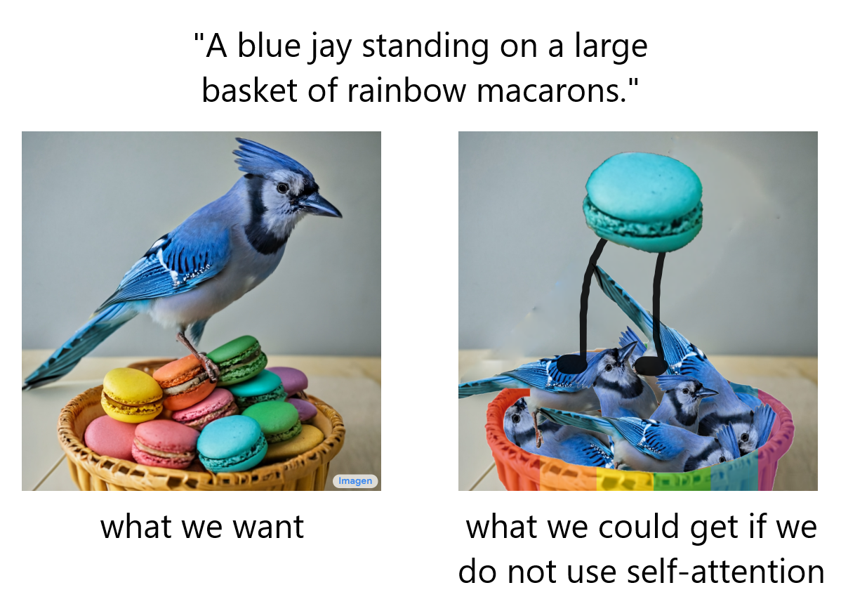
If Imagen only paid attention to individual words and not how they relate to one other, we could get high-quality images that capture individual elements of the caption, but do not portray them in a way that appropriately reflects the semantics of the caption. We can see this difference in the below example, where a lack of consideration for how words relate to one another could yield an extremely poor (albeit hilarious) result:

The text-encoder is frozen during training, meaning that it does not learn or change the way it creates the encodings. It is only used to generate encodings that are fed to the rest of the model, which is trained.

Now that we understand more about Imagen's text encoder, let's take a look at the component that actually generates images.

Image Generator

The text-encoder generates a useful representation of the caption input to Imagen, but we still need to devise a method to generate an image that uses this representation. To do this, Imagen uses a Diffusion Model, which is a type of generative model that has gained significant popularity in recent years due to its State-of-the-Art performance on several tasks. Before moving forward, let's look at a brief recap of Diffusion Models now.

What are Diffusion Models?

Diffusion Models are a method of creating data that is similar to a set of training data. They train by destroying the training data through the addition of noise, and then learning to recover the data by reversing this noising process. Given an input image, the Diffusion Model will iteratively corrupt the image with Gaussian noise in a series of timesteps, ultimately leaving pure Gaussian noise, or "TV static".

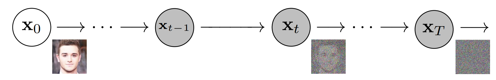
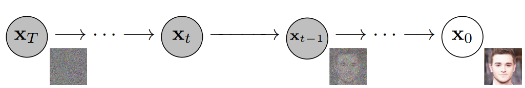
The Diffusion Model will then work backwards, learning how to isolate and remove the noise at each timestep, undoing the destruction process that just occurred.

Once trained, the model can then be "split in half", and we can start from randomly sampled Gaussian noise which we use the Diffusion Model to gradually denoise in order to generate an image.

Below we can see an example of handwritten digits being generated from pure Gaussian noise:

For a full treatment of Diffusion Models, feel free to check out our article covering them.

Caption Conditioning

To summarize, a trained Diffusion Model starts with Gaussian noise and then iteratively generates an image that is similar to the images on which it was trained. It may be apparent at this point that we have no control over what image is actually output - we simply input Gaussian noise into the model, and it spits out a random image that looks like it could belong to the training dataset. Recall that our goal is to create images that encapsulate the semantic information of the caption we input into Imagen, so we need a method of incorporating the caption into the diffusion process. How do we accomplish this?

Recall from above that our text encoder produced a representative encoding of the caption. This "encoding" is actually a sequence of vectors. To inject this encoding information into the Diffusion Model, we pool these vectors together and condition our diffusion model on them. By conditioning on this vector, the Diffusion Model learns how to adapt its denoising procedure in order to produce an image that is well-aligned with the caption. This process can be visualized in the video below:

Image Super-Resolution

The image generator, or "base" model, outputs a small 64x64 image. To upsample this model to the final 1024x1024 version we use a super-resolution model to intelligently upsample the image.

For the super-resolution model, Imagen again uses a Diffusion Model. The overall process is basically the same as the base model; except, instead of conditioning on just the caption encoding, we also condition on the smaller image which we are upsampling. The overall process can be visualized in the below video:

The output of this super-resolution model is actually not our final output but a medium sized image. To upscale this image to the final 1024x1024 resolution, yet another super-resolution model is used. The two super-resolution architectures are approximately equivalent, so we will not belabor the point by going into the details of the second super-resolution model.

The output of the second super-resolution model is the final output of Imagen.

Summary

To summarize, the caption is input into a pre-trained and frozen Transformer encoder which outputs a sequence of vectors (the text encoding). These vectors are important because they encode how words in the caption relate to one another and act as conditioning information for all other components of the model.

The text encodings are then passed into an image generation Diffusion Model, which starts with Gaussian noise and then gradually removes noise to generate a novel image which reflects the semantic information within the caption. The output of this model is a 64x64 pixel image.

After this, two more Diffusion Models are used to super-resolve this image to the final 1024x1024 size, again conditioned on the text encodings (as well as lower resolution images).

Now that we have a bird's-eye understanding of Imagen, we can dive into the details in the next section. Alternatively, feel free to jump down to the Results and Analysis or Final Words.

How Imagen Works: A Deep Dive

In the below sections, we will perform a Deep Dive into each of Imagen's components, highlighting certain structural features design-choice logic. We start with the text encoder.

Text Encoder

The text encoder in Imagen is the encoder network of T5 (Text-to-Text Transfer Transformer), a language model released by Google in 2019. T5 is a text-to-text model that serves as a general framework for many NLP tasks by framing them as text-to-text problems. We can see several examples of this approach in the below diagram, where translation, sentence-acceptability determination (cola), sentence-similarity estimation (stsb), and summarization are all cast in this manner.

T5 is intended to be finetuned for any NLP task that can be cast in this text-to-text manner.

Why is T5 Used in Imagen?

Some other text-to-image models like DALL-E 2 use text-encoders which are trained on image-caption pairs and an associated objective that is explicitly designed for the purpose of linking textual and visual representations of the same semantic concept. Such encoders, having been trained in an image-adjacent fashion, seem to therefore map more naturally to the problem of text-to-image generation than an NLP-specific text-encoder trained without regard to the image domain. It is therefore sensible to ask why the Imagen authors chose to use T5 as a text-encoder for Imagen.

The central intuition in using T5 is that extremely large language models, by virtue of their sheer size alone, may still learn useful representations despite the fact that they are not explicitly trained with any text/image task in mind. In addition to the extremely large size of some language models, it is also true that language models are trained on text-only corpi, which can be notably larger than datasets of paired text/images. The size and quality of a dataset that a model is trained on is arguably more important than the specifics of the model itself. In fact, T5 sees performance comparable to BERT even with only 25% of the training time thanks to its dataset. The combination of huge models and massive, diverse datasets leave plenty of headroom for learning powerful textual representations that may be useful in other domains.

Therefore, the central question being addressed by this choice is whether or not a massive language model trained on a massive dataset independent of the task of image generation is a worthwhile trade-off for a non-specialized text encoder. The Imagen authors bet on the side of the large language model, and it is a bet that seems to pay off well.

Image Generator

As mentioned above, the image generator in Imagen is a Diffusion Model, an unsurprising choice given their past few years of incredible progress. You can find a brief recap of Diffusion Models above or check out our dedicated Introduction to Diffusion Models for Machine Learning them for a full treatment.

With a basic understanding of Diffusion Models assumed, we will now explore the specifics of Imagen's implementation.

Network Architecture

A Diffusion Model is really sort of a "metamodel" framework that tells us how to use a neural model to denoise images. The architecture of the neural model itself has yet to be discussed or established, and the only relevant restriction on the neural model is that its input and output dimensionalities must be the same. That is, the image must not change size during the diffusion process.

With this restriction in mind, the authors select a U-Net architecture, as is common, which is left generally unmodified from the implementation by Nichol and Dhariwal. We can see the U-Net's overarching architecture below:

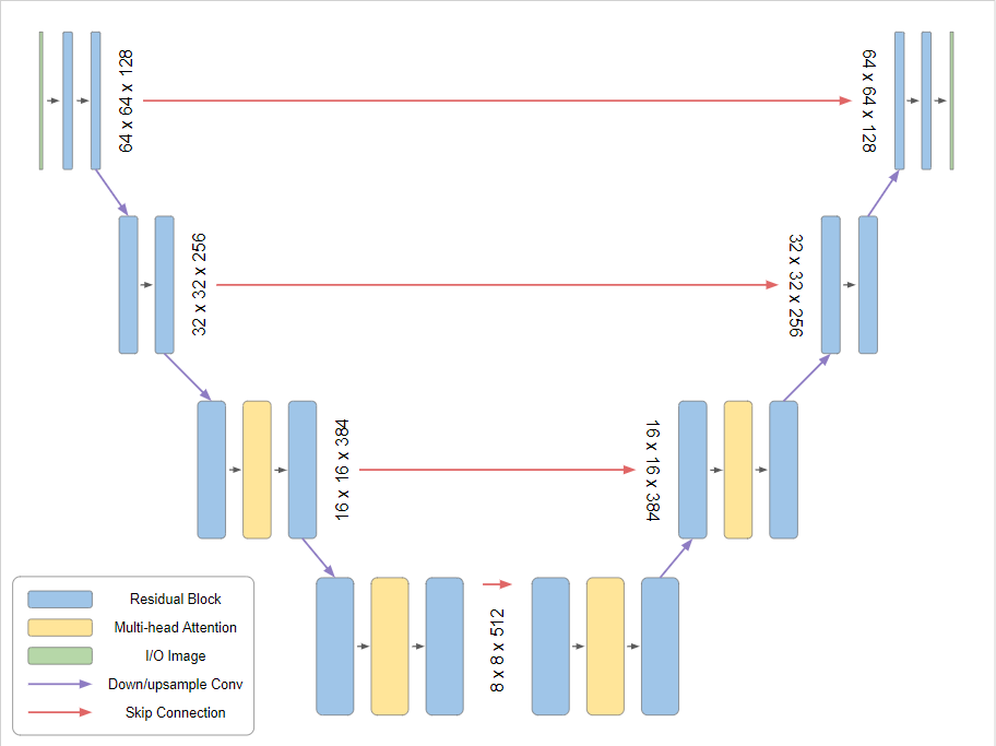
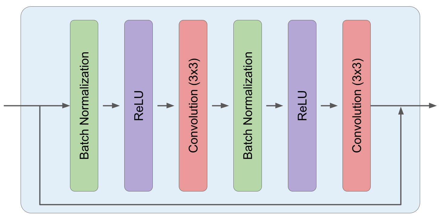
Each residual block is composed of two sub-blocks, and each of these sub-blocks is composed of a Batch Normalization, ReLU, and 3x3 Convolution in sequence.

Timestep Conditioning

In Imagen (and generally Diffusion Models as a whole), the same denoising U-Net is used at every timestep. Recall that different amounts of noise are removed at different timesteps in a Diffusion Model. We must therefore devise a way to inject timestep information into the model (i.e. condition on the timestep). The Imagen authors utilize a technique introduced by the original Transformer paper called positional encoding.

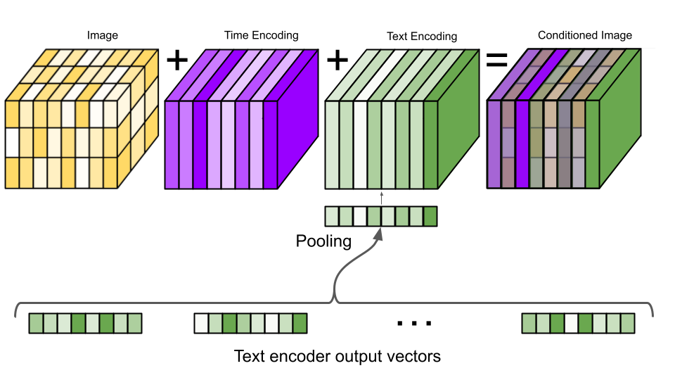
In Imagen, a unique timestep encoding vector is generated for each timestep (corresponding to "word position" in the original positional embedding implementation). At different resolutions in the U-Net, this vector is projected to having c components, where c is the number of channels in the U-Net at that resolution. After projection, each component of the vector is added to the corresponding channel (across its height and width) in the image.

This process is visualized below for the case of a 3x3 image with 8 channels:

While this is not exactly how timestep conditioning works in Imagen, it is very close and is in fact identical to how some other Diffusion Models inject timestep information. Note that some form of timestep encoding is required for any Diffusion Model (at least as they are commonly implemented) and is not unique to Imagen.

Caption Conditioning

We've yet to incorporate information from our image caption into the Diffusion Model U-Net, so we need to do that now. This caption conditioning happens in two ways.

First, the output vectors from the T5 text encoder are pooled and added into the timestep embedding from above. This process is visualized in the below image:

Next, the model is conditioned on the entire encoding sequence by adding cross attention over the text embeddings at several resolutions. The cross attention is implemented by concatenating the text embedding sequence to the key-value pairs of each self-attention layer.

Classifier-Free Guidance

Imagen also takes advantage of Classifier-Free Guidance. Classifier-Free Guidance is a method of increasing the image fidelity of a Diffusion Model at the cost of image diversity. The method is named as such due to the fact that it is a related and simpler version/extension of a previous method called Classifier Guidance, which was used for the same purposes.

Classifier Guidance

Classifier Guidance is a method for trading off the fidelity and diversity of images generated by a Diffusion Model. This method requires a trained classifier model, which is used to push the diffusion process towards feature regimes of high class probability. That is, the classifier is used to guide the image towards the classifier's own modes.

Consider the following equation:

If x is an image and y is a class label, then we can see that the gradient of the log probability density conditioned on the class label is equivalent to the unconditional log gradient plus a conditional term corresponding to the log gradient of the classifier. Scaling the conditional term is equivalent to pushing the weight of the classifier distribution towards its modes, encouraging the diffusion process towards images more likely for the given class. In the below video, you can see how pushing the weight of a Gaussian (blue) towards its mode affects its derivative at several points (red).

As mentioned before, the theoretical cost of this method is diversity, because images will be encouraged to have features that are frequently observed for the given class. The practical costs of this method are (1) needing to train a classifier in addition to the diffusion model, and (2) poor image quality when the conditional term is scaled too high (too high of a "guidance weight").

Classifier-Free Guidance works by training a Diffusion Model to be both conditional and unconditional at the same time. In order to do this, the Diffusion Model is cast as a conditional model and is trained with the conditioning information randomly dropped out a small fraction of the time (by replacing the conditional information with a NULL value). To use the model in an unconditional way, the NULL value is simply provided as the "conditional information" to the model.

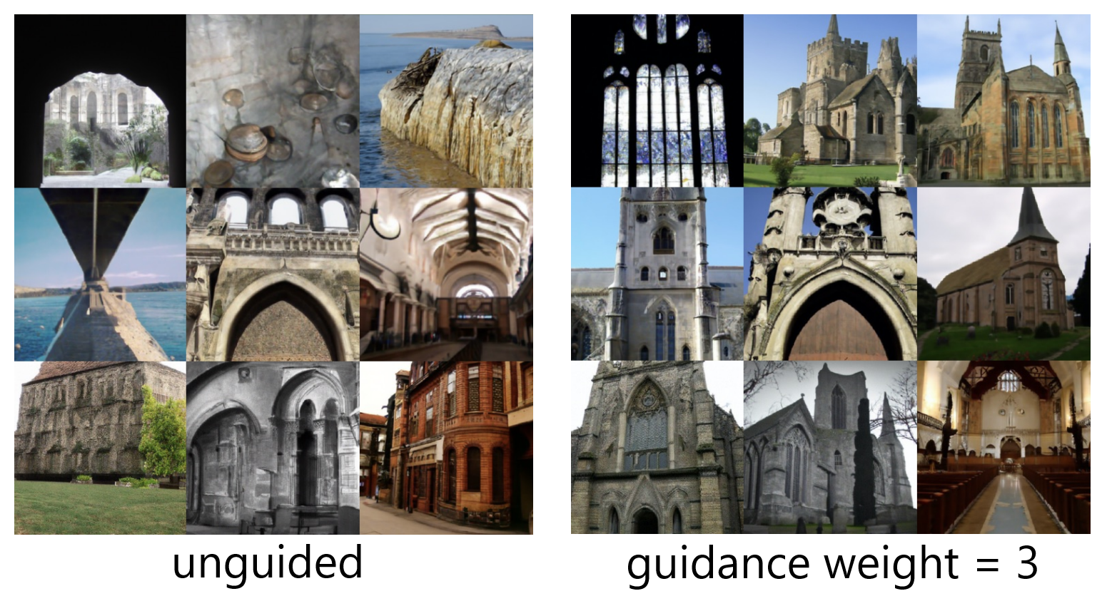
Given such a model, Classifier-Free guidance works loosely by interpolating between the unconditional and conditional gradients during inference. By magnifying the effect of the conditional gradient (i.e. making the "guidance weight" greater than 1), better samples can be obtained:

Although Classifier-Free Guidance was first introduced by Ho and Salimans, it was soon after notably used in OpenAI's GLIDE in order to create very high quality (albeit lower diversity) images. For a great resource on Classifier/Classifier-Free Guidance, check out this write-up.

According to Imagen's paper, Imagen depends critically on classifier-free guidance for effective text conditioning.

Large Guidance Weight Samplers

Classifier-Free Guidance is a very powerful way to improve the caption alignment of generated images, but it has been previously observed that extremely high guidance weights damage fidelity by yielding saturated and unnatural images.

The Imagen authors investigate this phenomenon and find that it arises from a train-test mismatch. In particular, the pixel values for the training data are scaled to the range [-1, 1], but high guidance weights cause the network outputs to exceed these bounds at given timestep. To make matters worse, since the same model is iteratively applied to its own output during diffusion, this effect compounds as the diffusion process proceeds, leading even potentially to divergence.

High guidance weights are found to be crucial for achieving State-of-the-Art image quality, so avoiding the problem by simply using lower guidance weights is not an option. Instead, the authors address the problem by devising two methods to threshold pixel values - static thresholding and dynamic thresholding. These methods address the train-test mismatch noted above and dynamic thresholding in particular is found to be critical to Imagen's performance.

Static Thresholding

In static thresholding, the pixel values at each timestep are simply clipped to the range [-1, 1]. This process can be visualized in the example below.

For the sale of example, let our pixel values be normally distributed. Applying static thresholding to these values means that any distribution weight that it outside of the pixel bounds (light red area) is pushed onto -1 for negative values and 1 for positive values. As we can see, as the variance of the distribution grows, the probability of being at an extreme value grows.

While this has some mitigating effect, images are unsurprisingly still oversaturated and less detailed as the guidance weight is increased. Therefore, the authors devised a better method of thresholding - dynamic thresholding.

Dynamic Thresholding

With dynamic thresholding, a certain percentile absolute pixel value is chosen. At each timestep, if that percentile value s exceeds 1, then the pixel values are thresholded to [-s, s] and divided by s. This process can be visualized in the below video:

Dynamic thresholding has the effect of bringing all pixel values back to the range [-1, 1], but operating on all pixels and not just those at the extreme. There is a "gravitational pull" back to 0 which balances the potential for divergence under an iteratively applied model.

The authors find that this method leads to much better photorealism and alignment, especially for large guidance weights.

Comparison

Below are several images depicting the effects of increasing the guidance weight for three models - one that is not thresholded, one that is statically thresholded, and one that is dynamically thresholded. Two distinct points ("pt1" and "pt2") are shown for each model and are the same between models. For each model and each point, several images are shown corresponding to different guidance weights (the only change).

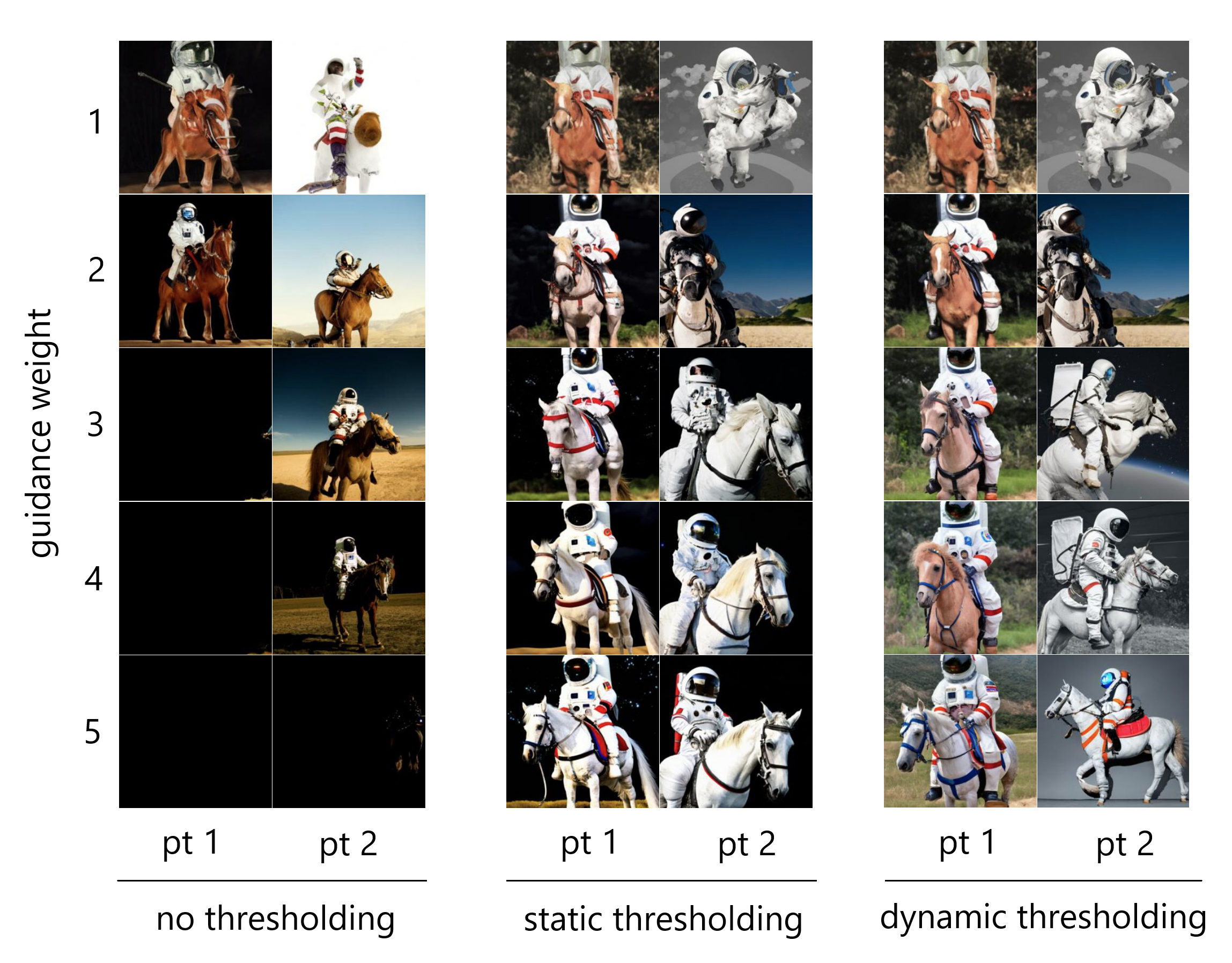
As we can see, static thresholding improves performance, at least yielding reasonable images for high guidance weights (even if saturated), unlike the unthresholded images which are almost completely black. Dynamic thresholding significantly improves performance, yielding reasonable and unsaturated images even to high guidance weights. While static and dynamic thresholding yield similar results at low guidance weights, differences in image saturation become more apparent at high guidance weights. These differences are especially evident when comparing the left columns of the two methods.

Super-Resolution Models

Recall that image generator Diffusion Model (or "base model") outputs 64x64 images. Imagen uses two conditional diffusion models to bring the image up to 1024x1024 resolution. Let's inspect these models now.

Small-to-Medium Architecture

The Small-to-Medium (STM) super-resolution model "takes in" (is conditioned on) the 64x64 image generated by the base model and super-resolves it to a 256x256 image. The STM model is yet another diffusion model, and is also conditioned on the caption encoding in addition to the low-resolution image. Cross-attention is implemented similarly to the base model.

The architecture of the STM model is another U-Net, again adapted from Nichol and Dhariwal like the Image Generator. The authors make several modifications to the model to improve memory efficiency, inference time, and convergence speed. They call this model Efficient U-Net, which is 2-3 times faster in steps/second than the unmodified version.

Medium-to-Large Architecture

The Medium-to-Large (MTL) super-resolution model super-resolves the 256x256 image generated by the STM model to a 1024x1204 image. The MTL model is very similar to the STM model, being a diffusion model that is conditioned on the caption encoding and the STM output image.

The architecture is generally similar to the STM model except that the self-attention layers are removed. Since there are no self-attention layers in this model, explicit cross-attention layers are added to attend over the text embeddings in contrast to the base and STM models.

Robust Cascaded Diffusion Models

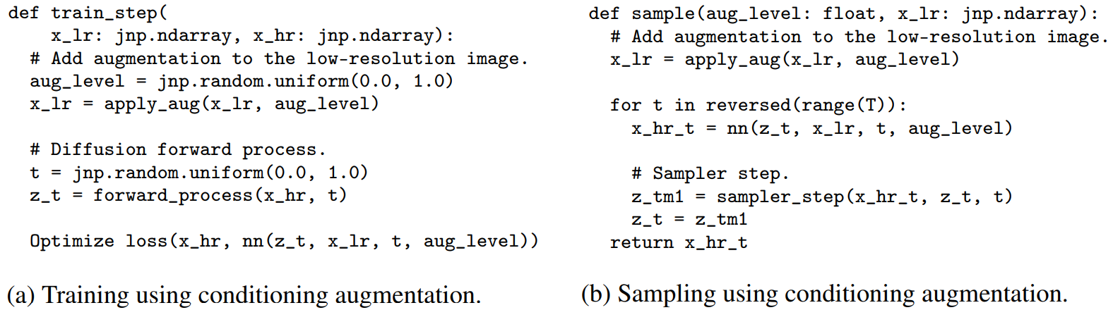
Imagen uses noise conditioning augmentation in the super-resolution models in order to make them aware of the amount of noise added. This conditioning improves sample quality and the ability of the models to handle artifacts resulting from the lower resolution models. The authors find this approach to be critical for generating high fidelity images.

The noise conditioning augmentation works by corrupting the low-resolution image upon which the super-resolution model is conditioned with Gaussian noise, and then conditioning the super-resolution model in addition on the corruption noise level. During training, the corruption noise level, or "augmentation level", is chosen randomly, whereas during inference this value is swept over to find the best sample quality.

The pseudocode for these processes can be seen below, where the authors are utilizing the JAX package.

Deep Dive Summary

To summarize, the input caption is fed into a T5 encoder, which is frozen during training. The text encoding conditions a base Diffusion Model, which uses a U-Net with self-attention layers at low resolutions to generate an image. The text encoding conditioning happens via addition to the timestep conditioning tensor ("positional encoding"), and via cross-attention through key-value concatenation to the self-attention layers. Dynamic thresholding and classifier-free guidance are implemented.

After the base model image has been generated, it is passed through two more Diffusion Models for super-resolution, which are conditioned on the images that they are upsampling in addition to conditioning on the timestep and text encoding. These models use noise conditioning augmentation to improve quality and remove artifacts.

The result is a 1024x1024 image that matches the input caption.

Results and Analysis

Quantitative

COCO is a dataset used to evaluate text-to-image models, with FID used to measure image fidelity and CLIP used to measure image-caption alignment. The authors find that Imagen achieves a State-of-the-Art zero-shot FID of 7.27 on COCO, outperforming DALL-E 2 and even models that were trained on COCO.

Qualitative

The authors note that both FID and CLIP have limitations. FID is not fully aligned with human perceptual quality, and CLIP is ineffective at counting. Therefore, they use human evaluation to assess quality and caption similarity, with 200 ground-truth caption-image pairs chosen at random from the COCO validation set used as a baseline. Subjects were shown batches of 50 of these images.

Quality

To probe the quality of Imagen's generated images, the human rater is asked to select between Imagen's generated image and a reference image using the question "Which image is more photorealistic (looks more real)?". The percentage of times raters choose Imagen's generated image over the reference image, called the preference rate is reported.

Imagen achieves a preference rate of 39.2% for photorealism.

Caption Similarity

To probe image-caption alignment, the rater is shown an image and a caption and asked "Does the caption accurately describe the above image?". The rater must respond with "yes", "somewhat", or "no". The responses are scored as 100, 50, and 0 respectively and obtained independently for model samples and references images, with both being reported.

The authors find that Imagen is on-par with original reference images for caption similarity.

DrawBench

Noting several shortcomings of COCO, the authors also introduce DrawBench - a comprehensive and challenging set of prompts that is intended to support the evaluation and comparison of text-to-image models.

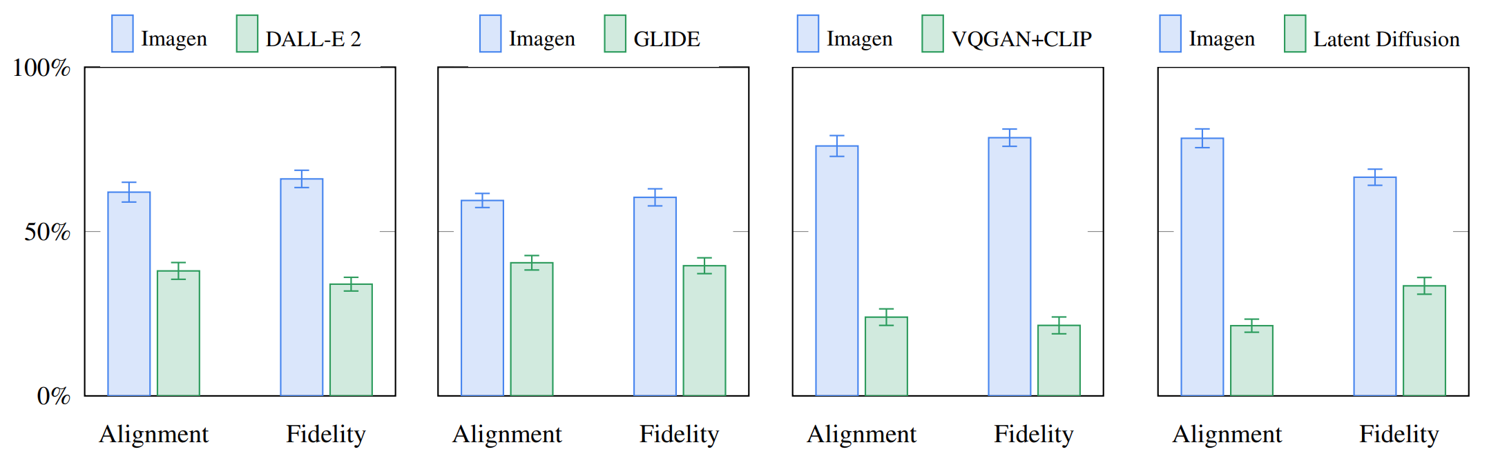
Below the results of comparing Imagen to DALL-E 2, GLIDE, VQGAN+CLIP, and Laten Diffusion on DrawBench are shown, where the bar heights correspond to user preference rates (with 95% confidence intervals) for both image fidelity and alignment. It is easy to see that Imagen outperforms all other models.

Why is Imagen Better than DALL-E 2?

Answering exactly why Imagen is better than DALL-E 2 is difficult; however, a non-negligible portion of the performance gap seems to stem from the differences in how the two models encode the caption/prompt.

DALL-E 2 uses a contrastive objective to determine how related a text encoding is to an image (essentially CLIP). The text and image encoders tune their parameters such that the cosine similarities of like caption-image pairs are maximized, while the cosine similarities of differing caption-image pairs are minimized. While this objective is very intuitive in the text-to-image domain, especially in reflection of the usage of the prior sub-model in DALL-E 2, what shortcomings does it have? We see three potential options.

Sheer Size

It may very well be that a notable portion of the performance gap stems from the fact that Imagen's text encoder is much larger than that of DALL-E 2's and is trained on more data. As evidence of this hypothesis, we can inspect the performance of Imagen as the text encoder is scaled up. Below we see pareto curves of Imagen's performance as a function of both encoder size as U-Net size.

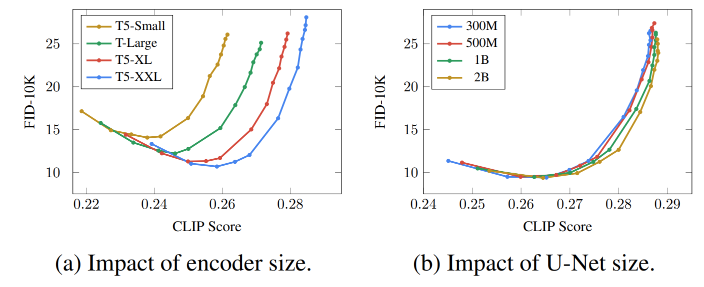
The effect of scaling up the text encoder is shockingly high, and that of scaling up the U-Net is shockingly low. This result suggests that relatively simple diffusion models can produce high-quality results as long as they are conditioned on powerful encodings.

Given that the T5 text encoder is so much larger than the CLIP text encoder, combined with the fact that natural language training data is necessarily more plentiful than image-caption pairs, much of the performance gap may be attributable to this difference, a fact which the Imagen authors note.

The Image Encoder Crutch

During CLIP training, both the text encoder and image encoder are tuned to satisfy the demands of the objective function. It is possible that there is a degree of freedom in how much each of these models are tuned in order to satisfy these demands. In particular, it may be the case that the image encoder in CLIP learns to produce richer encodings more quickly than the text encoder, adapting to the relatively lower performance of the text encoder. This would have the effect of lowering loss overall but simultaneously acting as a crutch to the text encoder. This crutch may lower the expressive power of the text encoder, leading to lower performance when repurposed for the purposes of DALL-E 2.

This observation is somewhat unintuitive. CLIP yields a space in which textual and visual manifestations of the same concepts are understood and mapped between with the prior in DALL-E 2. On the other hand, the responsibility of mapping textual encodings to visual concepts is put on the shoulders of the image generator in Imagen. Nevertheless, it may be the case that a weakened "starting point" for the prior in DALL-E 2 lowers the effectiveness of the prior, which ultimately propagates to the image generation sub-model.

Similar Concepts in Different Data Points

The next potential shortcoming of the CLIP text-encoding method is that the blanket objective of maximizing the cosine similarity of corresponding caption-image pairs while minimizing that of differing ones does not account for similar concepts in distinct data points. In particular, if two captions are very similar, they will properly be mapped to similar vectors, but the CLIP objective will push these vectors apart. To make matters worse, they will be pushed just as much apart as either of them together with a highly dissimilar caption vector. This penalty has the potential to weaken the learned encodings depending on the nature of the training dataset. Given the importance of the text encodings to text-to-image diffusion models, this behavior may weaken the quality of generated images.

While any of these factors may contribute to the performance gap, there are certainly other implementation details of Imagen that are relevant to our analysis, some of which are listed below in the "Key Takeaways" section.

Key Takeaways

Above notes regarding DALL-E 2 aside, the authors list several key takeaways from Imagen, including the following:

1. Scaling the text encoder is very effective
2. Scaling the text encoder is more important than U-Net size
3. Dynamic thresholding is critical
4. Noise conditioning augmentation in the super-resolution models is critical
5. Text conditioning via cross attention is critical
6. Efficient U-Net is critical

These insights provide valuable direction for other researchers who are working on Diffusion Models and are not useful only in the text-to-image subdomain.

Final Words

Imagen's results speak for themselves and mark another great success in the area text-to-image generation and generative modelling more generally. Imagen also adds to the list of the great accomplishments of Diffusion Models, which have taken the Machine Learning world by storm over the past few years with a string of absurdly impressive results.

Check out our article on Diffusion Models to learn more about them, or check out our article on DALL-E 2 to learn more about the previous king of text-to-image generation. Otherwise, feel free to follow our newsletter to stay in-the-loop for future articles like this.