
MinImagen - Build Your Own Imagen Text-to-Image Model
Text-to-Image models have made great strides this year, from DALL-E 2 to the more recent Imagen model. In this tutorial learn how to build a minimal Imagen implementation - MinImagen.


DALL-E 2 was released earlier this year, taking the world by storm with its impressive text-to-image capabilities. With just an input description of a scene, DALL-E 2 outputs realistic and semantically plausible images of the scene, like those you can see below generated from the input caption "a bowl of soup that is a portal to another dimension as digital art":

Just a month after DALL-E 2's release, Google announced a competing model Imagen that was found to be even better than DALL-E 2. Here are some example images:

The impressive results of both DALL-E 2 and Imagen rely on cutting-edge Deep Learning research. While necessary for attaining State-of-the-Art results, the usage of such cutting-edge research in models like Imagen renders them harder to understand for non-specialist researchers, in turn hindering the widespread adoption of these models and techniques.
Therefore, in the spirit of democratization, we will learn in this article how to build Imagen with PyTorch. In particular, we will construct a minimal implementation of Imagen - called MinImagen - that isolates the salient features of Imagen so that we can focus on understanding Imagen's integral operating principles, disentangling implementation aspects that are essential from those which are incidental.
Package Note
N.B. if you are not interested in implementation details and want only to use MinImagen, it has been packaged up and can be installed with
pip install minimagen
Check out the section below or the corresponding GitHub repository for usage tips. The documentation contains additional details and information about using the package.
Introduction
Text-to-image models have made great strides in the past few years, as evidenced by models like GLIDE, DALL-E 2, Imagen, and more. These strides are in large part due to the recent flourishing wave of research into Diffusion Models, a new paradigm/framework for generative models.
While there are some good resources on the theoretical aspects of Diffusion Models and text-to-image models, practical information on how to actually build these models is not as abundant. This is especially true for models that incorporate Diffusion Models as just one component of a larger system, common in text-to-image models, like the encoding-prior-generator chain in DALL-E 2, or the super-resolution chain in Imagen.
MinImagen strips off the bells and whistles of current best practices in order to isolate Imagen's salient features for educational purposes. The remainder of this article is structured as follows:
- Review of Imagen / Diffusion Models: In order to orient ourselves before we begin to code, we will briefly review both Imagen itself and Diffusion Models more generally. These reviews are intended to serve only as a refresher, so you should already have a working understanding of both of these topics when reading the refresher. You can check out our Introduction to Diffusion Models for Machine Learning and our dedicated guide to How Imagen Actually Works to learn more.
- Building the Diffusion Model: After our recap, we'll first build the
GaussianDiffusionclass in PyTorch, which defines the Diffusion Models used in Imagen. - Building the Denoising U-Net: We'll then build the denoising U-Net on which the Diffusion Models rely, manifested in the
Unetclass. - Building MinImagen: Next, we will put all of these pieces together using a T5 text encoder and a Diffusion Model chain in order to build our (Min)Imagen class,
Imagen. - Using MinImagen: Finally, we will learn how to train and sample from Imagen once it is fully defined.
Without further ado, it's time to jump into the recaps of both Imagen and Diffusion Models. If you are already familiar with Imagen and Diffusion Models from a theoretical perspective and want to jump to the PyTorch implementation details, click here.
What is Imagen?
Imagen is a text-to-image model that was released by Google just a couple of months ago. It takes in a textual prompt and outputs an image which reflects the semantic information contained within the prompt.

To generate an image, Imagen first uses a text encoder to generate a representative encoding of the prompt. Next, an image generator, conditioned on the encoding, starts with Gaussian noise ("TV static") and progressively denoises it to generate a small image that reflects the scene described by the caption. Finally, two super-resolution models sequentially upscale the image to higher resolutions, again conditioning on the encoding information.

The text encoder is a pre-trained T5 text encoder that is frozen during training. Both the base image generation model and the super-resolution models are Diffusion Models.
What is a Diffusion Model?
Diffusion Models are a class of generative models, meaning that they are used to generate novel data, often images. Diffusion Models train by corrupting training images with Gaussian Noise in a series of timesteps, and then learning to undo this noising process.

In particular, a model is trained to predict the noise component of an image at a given timestep.

Once trained, this denoising model can then be iteratively applied to randomly sampled Gaussian noise, "denoising" it in order to generate a novel image.

Diffusion Models constitute a sort of metamodel that orchestrates the training of another model - the noise prediction model. We therefore still have the task of deciding what type of model to actually use for the noise prediction itself. In general, U-Nets are chosen for this role. The U-Net in Imagen has a structure like this:

The architecture is based off of the model in the Diffusion Models Beat GANs on Image Synthesis paper. For MinImagen, we make some small changes to this architecture, including
- Removing the global attention layer (not pictured),
- Replacing the attention layers with transformer encoders, and
- Placing the transformer encoders at the end of the sequence at each layer rather than in between the residual blocks in order to allow for a variable number of residual blocks.
Build Your Own Imagen in PyTorch
With our Imagen/Diffusion Model recap complete, we are finally ready to start building out our Imagen implementation. To get started, first open up a terminal and clone the project repository:
git clone https://github.com/AssemblyAI-Examples/MinImagen.gitIn this tutorial, we will isolate the important parts of the source code that are relevant to the Imagen implementation itself, omitting details like argument validation, device handling, etc. Even a minimal implementation of Imagen is relatively large, so this approach is necessary in order to isolate instructive information. MinImagen's source code is thoroughly commented (with associated documentation here), so information regarding any omitted details should be easy to find.
Each big component of the project - the Diffusion Model, the Denoising U-Net, and Imagen - has been placed into its own section below. We'll start by building the GaussianDiffusion class.
Building the Diffusion Model
The Diffusion Model GaussianDiffusion class can be found in minimagen.diffusion_model. To jump to a summary of this section, click here.
Initialization
The GaussianDiffusion initialization function takes only one argument - the number of timesteps in the diffusion process.
class GaussianDiffusion(nn.Module):

    def __init__(self, *, timesteps: int):
    	super().__init__()
First, Diffusion Models require a variance schedule, which specifies the variance of the Gaussian noise that is added to image at a given timestep in the diffusion process. The variance schedule should be increasing, but there is some flexibility in how this schedule is defined. For our purposes we implement the variance schedule from the original Denoising Diffusion Probabilistic Models (DDPM) paper, which is a linearly spaced schedule from 0.0001 at t=0 to 0.02 at t=T.
class GaussianDiffusion(nn.Module):

    def __init__(self, *, timesteps: int):
    	super().__init__()

        self.num_timesteps = timesteps

        scale = 1000 / timesteps
        beta_start = scale * 0.0001
        beta_end = scale * 0.02
        betas = torch.linspace(beta_start, beta_end, timesteps, dtype=torch.float64)
From this schedule, we calculate a few values (again specified in the DDPM paper) that will be used in calculations later:

class GaussianDiffusion(nn.Module):

    def __init__(self, *, timesteps: int):
    	# ...

        alphas = 1. - betas
        alphas_cumprod = torch.cumprod(alphas, axis=0)
        alphas_cumprod_prev = F.pad(alphas_cumprod[:-1], (1, 0), value=1.)
The rest of the initialization function registers the above values and some derived values as buffers, which are like parameters except that they don't require gradients. All of the values are ultimately derived from the variance schedule and exist to make some calculations easier and cleaner down the line. The specifics of calculating the derived values are not important, but we will point out below any time one of these derived values is utilized.
Forward Diffusion Process
Now we can move on to define GaussianDiffusion's q_sample method, which is responsible for the forward diffusion process. Given an input image x_0, we noise it to a given timestep t in the diffusion process by sampling from the below distribution:

Sampling from the above distribution is equivalent to the below computation, where we have highlighted two of the buffers defined in __init__.

That is, the noisy version of the image at time t can be sampled by simply adding noise to the image, where both the original image and the noise are scaled by their respective coefficients as dictated by the timestep. Let's implement this calculation in PyTorch now by adding the method q_sample to the GaussianDiffusion class:
class GaussianDiffusion(nn.Module):

    def __init__(self, *, timesteps: int):
    	# ...

    def q_sample(self, x_start, t, noise=None):
        noise = default(noise, lambda: torch.randn_like(x_start))

        noised = (
                extract(self.sqrt_alphas_cumprod, t, x_start.shape) * x_start +
                extract(self.sqrt_one_minus_alphas_cumprod, t, x_start.shape) * noise
        )

        return noised
x_start is a PyTorch tensor of shape (b, c, h, w), t is a PyTorch tensor of shape (b,) that gives, for each image, the timestep to which we would like to noise each image to, and noise allows us to optionally supply custom noise rather than sample Gaussian noise.
We simply perform and return the calculation in the equation above, using elements from the aforementioned buffers as coefficients. The default function samples random Gaussian noise when None is supplied, and extract extracts the proper values from the buffers according to t.
Reverse Diffusion Process
Ultimately, our goal is to sample from this distribution:

Given an image and its noised counterpart, this distribution tells us how to take a step "back in time" in the diffusion process, slightly denoising the noisy image. Similarly to above, sampling from this distribution is equivalent to calculating

To perform this calculation, we require the distribution's mean and variance. The variance is a deterministic function of the variance schedule:

On the other hand, the mean depends on the original and noised images (although the coefficients are again deterministic functions of the variance schedule). The form of the mean is:

At inference, we will not have x_0, the "original image", because it is what we are trying to generate (a novel image). This is where our trainable U-Net comes into the picture - we use it to predict x_0 from x_t.
In practice, better results are seen when the U-Net learns to predict the noise component of the image, from which we can calculate x_0. Once we have x_0, we can calculate the distribution mean with the formula above, giving us what we need to sample from the posterior (i.e. denoise the image back one timestep). Visually, the overall process looks like this:

The function to sample from the posterior (green block in the diagram) will be defined in the Imagen class, but we will define the two remaining functions now. First, we implement the function that calculates x_0 given a noised image and its noisy component (red block in the diagram). From above, we have:

Rearranging it in order to isolate x_0 yields the below, where two buffers have again been highlighted.

That is, to calculate x_0 we simply subtract the noise (predicted by the U-Net) from x_t, where both noisy image and noise itself are scaled by their respective coefficients as dictated by the timestep. Let's implement this function predict_start_from_noise in PyTorch now:
class GaussianDiffusion(nn.Module):

    def __init__(self, *, timesteps: int):
    	# ...

    def q_sample(self, x_start, t, noise=None):
        # ...

    def predict_start_from_noise(self, x_t, t, noise):
        return (
                extract(self.sqrt_recip_alphas_cumprod, t, x_t.shape) * x_t -
                extract(self.sqrt_recipm1_alphas_cumprod, t, x_t.shape) * noise
        )
Now that we have a function for calculating x_0, we can go back and calculate the posterior mean and variance (yellow block in the diagram). We repeat below their functional definitions from above, highlighting buffers defined in _init__ as needed.


Let's implement a function q_posterior to calculate these variables in PyTorch:
class GaussianDiffusion(nn.Module):

    def __init__(self, *, timesteps: int):
    	# ...

    def q_sample(self, x_start, t, noise=None):
        # ...

    def predict_start_from_noise(self, x_t, t, noise):
        return (
                extract(self.sqrt_recip_alphas_cumprod, t, x_t.shape) * x_t -
                extract(self.sqrt_recipm1_alphas_cumprod, t, x_t.shape) * noise
        )

    def q_posterior(self, x_start: torch.tensor, x_t: torch.tensor, t: torch.tensor, **kwargs):
        posterior_mean = (
                extract(self.posterior_mean_coef1, t, x_t.shape) * x_start +
                extract(self.posterior_mean_coef2, t, x_t.shape) * x_t
        )
        posterior_variance = extract(self.posterior_variance, t, x_t.shape)
        posterior_log_variance_clipped = extract(self.posterior_log_variance_clipped, t, x_t.shape)
        return posterior_mean, posterior_variance, posterior_log_variance_clipped
In practice, we return both the variance and log of the variance (posterior_log_variance_clipped, where "clipped" means that we push values of 0 to 1e-20 before taking the log). The reason for using the log of the variance is numerical stability in our calculations, which we will point out later when relevant.
Summary
To recap, in this section we defined the GaussianDiffusion class, which is responsible for defining the diffusion process operations. We first implemented q_sample, which performs the forward diffusion process, noising images to a given timestep in the diffusion process. We also implemented predict_start_from_noise and q_posterior, which are used to calculate parameters that are used in the reverse diffusion process.
Building the Noise Prediction Model
Now it's time to denoise our noise prediction model - the U-Net. This model is fairly complicated, so to be concise we will examine its forward pass, introducing relevant objects in the __init__ where relevant. Examining only the forward pass will help us understand how the U-Net works operationally while omitting unnecessary details that are not instructive in our learning how to build Imagen.
The U-Net class Unet can be found in minimagen.Unet. To jump to a summary of this section, click here.
Overview
Recall that the U-Net architecture for Imagen is similar to the one seen in the below diagram. We make a few modifications, most notably placing the attention block (which is a Transformer encoder for us) at the end of each layer in the U-Net.
Generating Time Conditioning Vectors
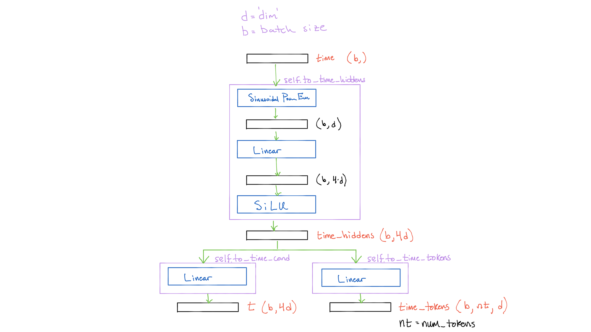
Remember that our U-Net is a conditional model, meaning it depends on our input text captions. Without this conditioning, there would be no way to tell the model what we want to be present in the generated images. Additionally, since we are using the same U-Net for all timesteps, we need to condition on the timestep information so the model knows what magnitude of noise it should be removing at any given time (remember, our variance schedule varies with t). Let's take a look at how we generate this time conditioning signal now. A diagram of these calculations can be seen at the end of this section.
Input to the model we receive a time vector of shape (b,), which provides the timestep for each image in the batch. We first pass this vector through a module which generates hidden states from them:
class Unet(nn.Module):
    def __init__(self, *args, **kwargs):
    	# ...

        self.to_time_hiddens = nn.Sequential(
            SinusoidalPosEmb(dim),
            nn.Linear(dim, time_cond_dim),
            nn.SiLU()
        )

    def forward(self, *args, **kwargs):

    	time_hiddens = self.to_time_hiddens(time)
First, for each time a unique positional encoding vector is generated (SinusoidalPostEmb()), which maps the integer value of the timestep for a given image into a representative vector that we can use for timestep conditioning. For a recap on positional encodings, see the dropdown here. Next, these encodings are projected to a higher dimensional space (time_cond_dim), and passed through the SiLU nonlinearity. The result is a tensor of size (b, time_cond_dim) that constitutes our hidden states for the timesteps.
These hidden states are then used in two ways. First, a time conditioning tensor t is generated, which we will use to provide timestep conditioning at each step in the U-Net. These are generated from time_hiddens with a simple linear layer. Second, time tokens time_tokens are generated again from time_hiddens with a simple linear layer, which are concatenated to the main text-conditioning tokens we will generate momentarily. The reason we have these two uses is because the time conditioning is necessarily provided everywhere in the U-Net (via simple addition), while the main conditioning tokens are used only in the cross-attention operation in specific blocks/layers of the U-Net. Let's see how to implement these functions in PyTorch:
class Unet(nn.Module):
    def __init__(self, *args, **kwargs):
    	# ...

        self.to_time_cond = nn.Sequential(
            nn.Linear(time_cond_dim, time_cond_dim)
        )

        self.to_time_tokens = nn.Sequential(
            nn.Linear(time_cond_dim, cond_dim * NUM_TIME_TOKENS),
            Rearrange('b (r d) -> b r d', r=NUM_TIME_TOKENS)
        )

    def forward(self, *args, **kwargs):
    	# ...
        t = self.to_time_cond(time_hiddens)
        time_tokens = self.to_time_tokens(time_hiddens)
The shape of t is (b, time_cond_dim), the same as time_hiddens. The shape of time_tokens is (b, NUM_TIME_TOKENS, cond_dim), where NUM_TIME_TOKENS defines how many time tokens should be generated that will be concatenated on the main conditioning text tokens. The default value is 2. The einops Rearrange layer reshapes the tensor from (b, NUM_TIME_TOKENS*cond_dim) to (b, NUM_TIME_TOKENS, cond_dim).
The time encoding process is summarized in this figure:

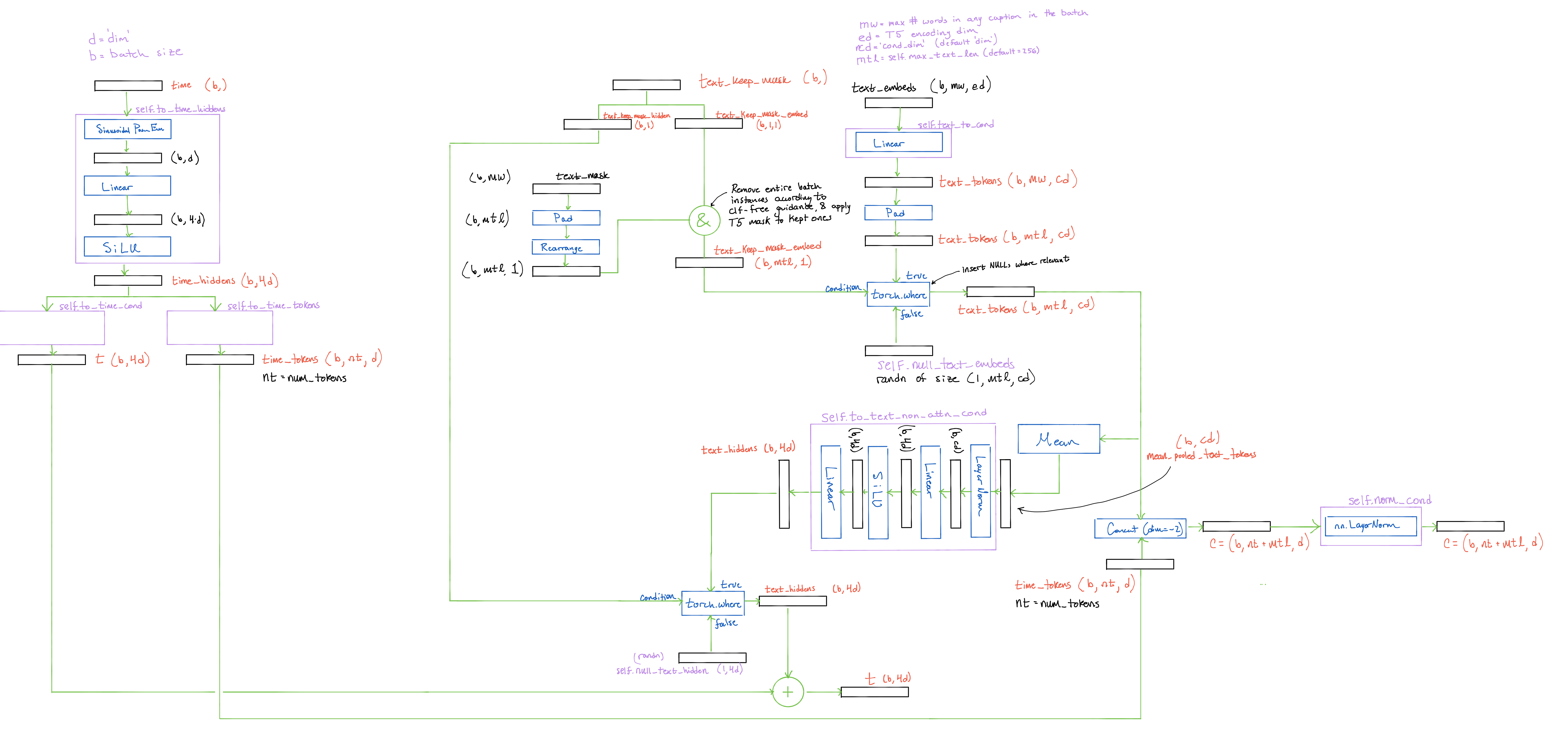
Generating Text Conditioning Vectors
Now it is time to generate our text conditioning objects. From our text encoder we have two tensors - the text embeddings of the batch captions, text_embeds, and the text mask, text_mask, which tells us how many words are in each caption in the batch. These tensors are size (b, max_words, enc_dim), and (b, max_words) respectively, where max_words is the number of words in the longest caption in the batch, and enc_dim is the encoding dimension of the text encoder.
We also incorporate classifier-free guidance at this point; so, given all of the moving parts, let's take a look at a visual example to understand what's going at a high level. All of the calculations are again summarized in a diagram below.
Visual Example
Let's assume that we have three captions - 'a very big red house', 'a man', and 'a happy dog'. Our text encoder provides the following:

We project the embedding vectors to a higher dimension (greater horizontal width), and pad both the mask and embedding tensors (extra entry vertically) to the maximum number of words allowed in a caption, a value we choose and which we let be 6 here:

From here, we incorporate classifier-free guidance by randomly deciding which batch instances to drop with a fixed probability. Let's just assume that the last instance is dropped, which is implemented by alterting the text mask.

Continuing with classifier-free guidance, we generate NULL vectors to use for the dropped elements.

We replace the encodings will NULL wherever the text mask is red:

To get the final main conditioning token c, we simple concatenate the time_tokens generated above to these text conditioning tensors. The concatenation happens along the num_tokens/word dimension to leave a final main conditioning token of shape (b, NUM_TIME_TOKENS + max_text_len, cond_dim).
Finally, we also mean pool across the word dimension to acquire a tensor of shape (b, cond_dim), and then project to the time conditioning vector dimension to yield a tensor of shape (b, 4*cond_dim). After dropping the necessary instances along the batch dimensions according to the classifier-free guidance vector, we add this to t to get the final timestep conditioning t.
Corresponding Code
The corresponding code for these operations is a bit cumbersome and just reiterates/implements the above process, so the code will be omitted here. Feel free to check out the Unet._text_condition method in the source code to explore how this function is implemented. The below image summarizes the entire conditioning generation process, so feel free to open this image in a new tab and follow along visually while going through the code in order to stay oriented.

Building the U-Net
Now that we have the two conditioning tensors we need - the main conditioning tensor c applied via attention and the time conditioning tensor t applied via addition - we can move on to defining the U-Net itself. As above, we continue by examining Unet's forward method, introducing objects in __init__ as needed.
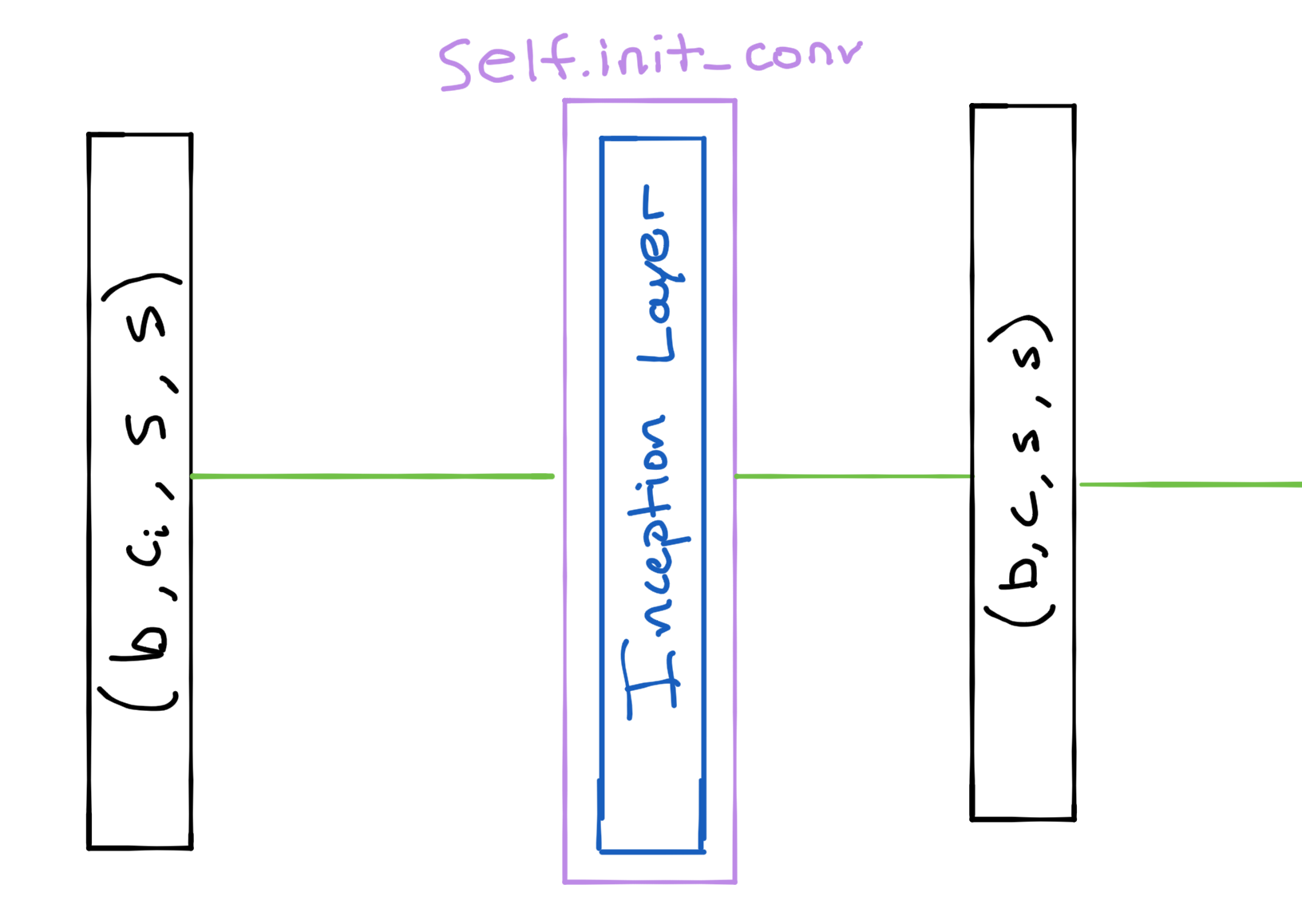
Initial Convolution
First, we need to perform an initial convolution to get our input images to the expected number of channels for the network. We utilize minimagen.layers.CrossEmbedLayer, which is essentially an Inception layer.
class Unet(nn.Module):
    def __init__(self, *args, **kwargs):
    	# ...
        self.init_conv = CrossEmbedLayer(channels, dim_out=dim, kernel_sizes=(3, 7, 15), stride=1)

    def forward(self, *args, **kwargs):
    	# ...
        x = self.init_conv(x)
Initial ResNet Block
Next, we pass the images into the initial ResNet block (minimagen.layers.ResnetBlock) for this layer of the U-Net, called init_block.
class Unet(nn.Module):
    def __init__(self, *args, **kwargs):
    	# ...
        self.init_block = ResnetBlock(current_dim, current_dim, cond_dim=layer_cond_dim, time_cond_dim=time_cond_dim, groups=groups)

    def forward(self, *args, **kwargs):
    	# ...
        x = init_block(x, t, c)
The ResNet block first passes the images through an initial block1 (minimagen.layers.block), resulting in an output tensor of the same size as the input.

Next, residual cross attention (minimagen.layers.CrossAttention) is performed with the main conditioning tokens

After that we pass the time encodings through a simple MLP to attain the proper dimensionality, and then split it into two sizes (b, c, 1, 1) tensors.

We finally pass the images through another convolution block that is identical to block1, except for the fact that it incorporates the timestep information via a scale-shift using the timestep embeddings.

The final resulting output of init_block has the same shape as the input tensor.
Remaining ResNet Blocks
Next, we pass the images through a sequence of ResNet blocks that are identical to init_block, except for the fact that they only condition on the timestep. We save the outputs in hiddens for the skip connections later on.
class Unet(nn.Module):
    def __init__(self, *args, **kwargs):
    	# ...
        self.resnet_blocks = nn.ModuleList(
                    [
                        ResnetBlock(current_dim, current_dim, time_cond_dim=time_cond_dim, groups=groups)
                        for _ in range(layer_num_resnet_blocks)
                    ]

    def forward(self, *args, **kwargs):
    	# ...
        hiddens = []
        for resnet_block in self.resnet_blocks:
                x = resnet_block(x, t)
                hiddens.append(x)
Final Transformer Block
After processing with the ResNet blocks, we optionally pass the images through a Transformer encoder (minimagen.layers.TransformerBlock).
class Unet(nn.Module):
    def __init__(self, *args, **kwargs):
    	# ...
        self.transformer_block = TransformerBlock(dim=current_dim, heads=ATTN_HEADS, dim_head=ATTN_DIM_HEAD)

    def forward(self, *args, **kwargs):
    	# ...
        x = self.transformer_block(x)
        hiddens.append(x)
The transformer block applies multi-headed attention (purple block below), and then passes the output through a minimagen.layers.ChanFeedForward layer, a sequence of convolutions with layer norms between them and GeLU between them.
Detailed Diagram
Downsample
As the final step for this layer of the U-Net, the images are downsampled to half the spatial width.
class Unet(nn.Module):
    def __init__(self, *args, **kwargs):
    	# ...
        self.post_downsample = Downsample(current_dim, dim_out)

    def forward(self, *args, **kwargs):
    	# ...
        x = post_downsample(x)
Where the downsampling operation is a simple fixed convolution.
def Downsample(dim, dim_out=None):
    dim_out = default(dim_out, dim)
    return nn.Conv2d(dim, dim_out, kernel_size=4, stride=2, padding=1)
Middle Layers
The above sequence of ResNet blocks, (possible) Transformer encoder, and Downsampling is repeated for each layer of the U-Net until we reach the lowest spatial resolution / greatest channel depth. At this point, we pass the images through two more ResNet blocks, which do condition on the main conditioning tokens (like the init_block of each Resnet Layer). Optionally, we pass the images through a residual Attention layer between these blocks.
class Unet(nn.Module):
    def __init__(self, *args, **kwargs):
    	# ...
                self.mid_block1 = ResnetBlock(mid_dim, mid_dim, cond_dim=cond_dim, time_cond_dim=time_cond_dim,
                                      groups=resnet_groups[-1])
        self.mid_attn = EinopsToAndFrom('b c h w', 'b (h w) c',
                                        Residual(Attention(mid_dim, heads=ATTN_HEADS,
                                                           dim_head=ATTN_DIM_HEAD))) if attend_at_middle else None
        self.mid_block2 = ResnetBlock(mid_dim, mid_dim, cond_dim=cond_dim, time_cond_dim=time_cond_dim,
                                      groups=resnet_groups[-1])

    def forward(self, *args, **kwargs):
    	# ...
        x = self.mid_block1(x, t, c)
        if exists(self.mid_attn):
            x = self.mid_attn(x)
        x = self.mid_block2(x, t, c)
Upsampling Trajectory
The upsampling trajectory of the U-Net is largely a mirror-inverse of the downsampling trajectory, except for the fact that we (a) concatenate the corresponding skip connections from the downsampling trajectory before each resnet block at any given layer, and (b) we use an upsampling operation rather than a downsampling one. This upsampling operation is a nearest-neighbor upsampling followed by a spatial size preserving convolution
def Upsample(dim, dim_out=None):
    dim_out = default(dim_out, dim)

    return nn.Sequential(
        nn.Upsample(scale_factor=2, mode='nearest'),
        nn.Conv2d(dim, dim_out, 3, padding=1)
    )
For the sake of brevity, the upsampling trajectory code is not repeated here, but can be found in the source code.
At the end of the upsampling trajectory, a final convolution layer brings the images to the proper output channel depth (generally 3).
Summary
To recap, in this section we defined the Unet class, which is responsible for defining the denoising U-Net that is trained via Diffusion. We first learned how to generate conditioning tensors for a given timestep and caption, and then incorporate this conditioning information into the U-Net's forward pass, which sends images through a series of ResNet blocks and Transformer encoders in order to predict the noise component of a given image
Building Imagen
To recap, we have constructed a GaussianDiffusion object which defines and implements the diffusion process "metamodel", which in turn utilizes our Unet class to train. Let's now take a look at how we put these pieces together to build Imagen itself. We'll again look at the two primary functions within Imagen - forward for training and sample for image generation, again introducing objects in __init__ as needed.
The Imagen class can be found in minimagen.Imagen. To jump to a summary of this section, click here.
Imagen Forward Pass
The Imagen forward pass consists of (1) noising the training images, (2) predicting the noise components with the U-Net, and then (3) returning the loss between the predicted noise and the true noise.
To begin, we randomly sample timesteps to noise the training images to, and then encoding the conditioning text, placing the embeddings and masks on the same device as the input image tensor:
from minimagen.t5 import t5_encode_text

class Imagen(nn.Module):
    def __init__(self, timesteps):
        self.noise_scheduler = GaussianDiffusion(timesteps=timesteps)
        self.text_encoder_name = 't5_small'

    def forward(self, images, texts):
        times = self.noise_scheduler.sample_random_times(b, device=device)

        text_embeds, text_masks = t5_encode_text(texts, name=self.text_encoder_name)
        text_embeds, text_masks = map(lambda t: t.to(images.device), (text_embeds, text_masks))
Recall that Imagen has a base model that generates small images and super-resolution models that upscale the images. We therefore need to resize the images to the proper size for the U-Net in use. If the U-Net is a super-resolution model, we additionally need to rescale the training images first down to the low-resolution conditioning size, and then up to the proper size for the U-Net. This simulates the upsampling of one U-Net's output to the size of the next U-Net's input in Imagen's super-resolution chain (allowing the latter U-Net to condition on the former U-Net's output).
We also add noise to the low-resolution conditioning images for noise conditioning augmentation, picking one noise level for the whole batch.
#...
from minimagen.helpers import resize_image_to
from einops import repeat

class Imagen(nn.Module):
    def __init__(self, timesteps):
    	# ...
        self.lowres_noise_schedule = GaussianDiffusion(timesteps=timesteps)


    def forward(self, images, texts):
    	# ...
        lowres_cond_img = lowres_aug_times = None
        if exists(prev_image_size):
            lowres_cond_img = resize_image_to(images, prev_image_size, pad_mode='reflect')
            lowres_cond_img = resize_image_to(lowres_cond_img, target_image_size,
            					pad_mode='reflect')

            lowres_aug_time = self.lowres_noise_schedule.sample_random_times(1, device=device)
            lowres_aug_times = repeat(lowres_aug_time, '1 -> b', b=b)

        images = resize_image_to(images, target_image_size)
Finally, we calculate and return the loss:
#...
from minimagen.helpers import resize_image_to
from einops import repeat

class Imagen(nn.Module):
    def __init__(self, timesteps):
    	# ...

    def forward(self, images, texts, unet):
    	# ...
        return self._p_losses(unet, images, times, text_embeds=text_embeds,
        			text_mask=text_masks,
                            	lowres_cond_img=lowres_cond_img,
                            	lowres_aug_times=lowres_aug_times)
Let's take a look at _p_losses to see how we calculate the loss.
First, we use the Diffusion Model forward process to noise both the input images and, if the U-Net is a super-resolution model, the low-resolution conditioning images as well.
#...

class Imagen(nn.Module):
    def __init__(self, timesteps):
    	# ...

    def p_losses(self, x_start, times, lowres_cond_img=None):
    	# ...
        noise = torch.randn_like(x_start)

        x_noisy = self.noise_scheduler.q_sample(x_start=x_start, t=times, noise=noise)

        lowres_cond_img_noisy = None
        if exists(lowres_cond_img):
            lowres_aug_times = default(lowres_aug_times, times)
            lowres_cond_img_noisy = self.lowres_noise_schedule.q_sample(
                            		x_start=lowres_cond_img, t=lowres_aug_times,
                        		noise=torch.randn_like(lowres_cond_img))
Next, we use the U-Net to predict the noise component of the noisy images, taking in text embeddings as conditioning information, in addition to the low-resolution images if the U-Net is for super-resolution. cond_drop_prob gives the probability of dropout for classifier-free guidance.
#...

class Imagen(nn.Module):
    def __init__(self, timesteps):
    	# ...
        self.cond_drop_prob = 0.1

    def p_losses(self, x_start, times, text_embeds, text_mask, lowres_cond_img=None):
    	# ...
        pred = unet.forward(
            x_noisy,
            times,
            text_embeds=text_embeds,
            text_mask=text_mask,
            lowres_noise_times=lowres_aug_times,
            lowres_cond_img=lowres_cond_img_noisy,
            cond_drop_prob=self.cond_drop_prob,
        )
We then calculate the loss between the actual noise that was added and the U-Net's prediction of the noise according to self.loss_fn, which is L2 loss by default.
#...

class Imagen(nn.Module):
    def __init__(self, timesteps):
    	# ...
        self.loss_fn = torch.nn.functional.mse_loss

    def p_losses(self, x_start, times, text_embeds, text_mask, lowres_cond_img=None):
    	# ...
        return self.loss_fn(pred, noise)
That's all it takes to get the loss with Imagen! It is quite a simple process once we have built the Diffusion Model/U-Net backbone.
Sampling with Imagen
Ultimately, what we want to do is sample with Imagen. That is, we want to be able to generate novel images given textual captions. Recall from above that this requires calculating the forward process posterior mean:
Now that we have defined our U-Net that predicts the noise component, we have all of the pieces we need to compute the posterior mean.
First, we get the noise prediction (blue) using our U-Net's forward (or forward_with_cond_scale) method, and then calculate x_0 from it (red) using the U-Net's predict_start_from_noise method introduced previously which performs the below calculation:

Where x_t is a noisy image and epsilon is the U-Net's noise prediction. Next, x_0 is dynamically thresholded and then passed, along with x_t, into the into the q_posterior method of the U-Net (yellow) to get the distribution mean.
This whole process is wrapped up in Imagen's _p_mean_variance function.
From here we have everything we need to sample from the posterior, which is to say "go back one timestep" in the diffusion process. That is, we are seeking to sample from the below distribution:
#...

class Imagen(nn.Module):
    def __init__(self, timesteps):
    	# ...
        self.dynamic_thresholding_percentile = 0.9


    def _p_mean_variance(self, unet, x, t, *, noise_scheduler
    			text_embeds=None, text_mask=None):

        # Get the noise prediction from the unet (blue block)
        pred = unet.forward_with_cond_scale(x, t, text_embeds=text_embeds, text_mask=text_mask)

        # Calculate the starting images from the noise (yellow block)
        x_start = noise_scheduler.predict_start_from_noise(x, t=t,

        # Dynamically threshold
        s = torch.quantile(
            rearrange(x_start, 'b ... -> b (...)').abs(),
            self.dynamic_thresholding_percentile,
            dim=-1
        )

        s.clamp_(min=1.)
        s = right_pad_dims_to(x_start, s)
        x_start = x_start.clamp(-s, s) / s

        # Return the forward process posterior parameters (green block)
        return noise_scheduler.q_posterior(x_start=x_start, x_t=x, t=t, t_next=t_next)
We saw above that sampling from this distribution is equivalent to calculating
Since we calculated the posterior mean and (log) variance with _p_mean_variance, we can now implement the above calculation with _p_sample, calculating the square root of the variance as such for numerical stability.
class Imagen(nn.Module):
    def __init__(self, timesteps):
    	# ...
        self.dynamic_thresholding_percentile = 0.9

    @torch.no_grad()
    def _p_sample(self, unet, x, t, *, text_embeds=None, text_mask=None):

        b, *_, device = *x.shape, x.device

        # Get posterior parameters
        model_mean, _, model_log_variance = self.p_mean_variance(unet, x=x, t=t,
        					text_embeds=text_embeds, text_mask=text_mask)

        # Get noise which we will use to calculate the denoised image
        noise = torch.randn_like(x)

        # No more denoising when t == 0
        is_last_sampling_timestep = (t == 0)
        nonzero_mask = (1 - is_last_sampling_timestep.float()).reshape(b,
        							*((1,) * (len(x.shape) - 1)))

        # Get the denoised image. Equivalent to mean * sqrt(variance) but calculate this way to be more numerically stable
        return model_mean + nonzero_mask * (0.5 * model_log_variance).exp() * noise
At this point, we have denoised the random noise input into Imagen one timestep. To generate images, we need to do this for every timestep, starting with randomly sampled Gaussian noise at t=T and going "back in time" until we reach t=0. Therefore, we run _p_sample in a loop over timesteps with _p_sample_loop:
class Imagen(nn.Module):
    def __init__(self, *args, **kwargs):
    	# ...

    @torch.no_grad()
    def p_sample_loop(self, unet, shape, *, lowres_cond_img=None, lowres_noise_times=None,
    			noise_scheduler=None, text_embeds=None, text_mask=None):

        device = self.device

        # Get starting noisy images
        img = torch.randn(shape, device=device)

	# Get sampling timesteps (final_t, final_t-1, ..., 2, 1, 0)
	batch = shape[0]
        timesteps = noise_scheduler.get_sampling_timesteps(batch, device=device)

	# For each timestep, denoise the images slightly
        for times in tqdm(timesteps, desc='sampling loop time step', total=len(timesteps)):
            img = self.p_sample(
                unet,
                img,
                times,
                text_embeds=text_embeds,
                text_mask=text_mask)

	# Clamp the values to be in the allowed range and potentialy
   	# unnormalize back into the range (0., 1.)
        img.clamp_(-1., 1.)
        unnormalize_img = self.unnormalize_img(img)
        return unnormalize_img
_p_sample_loop is how we generate images with one unet. Imagen contains a chain of U-Nets, so, finally, the sample function iteratively passes the generated images through each U-Net in the chain, and handles other sampling requirements like generating text encodings/masks, placing the currently-sampling U-Net on the GPU if available, etc. eval_decorator sets the model to be in evaluation mode if it is not upon calling sample.
class Imagen(nn.Module):
    def __init__(self, *args, **kwargs):
    	# ...
        self.noise_schedulers = nn.ModuleList([])
        for i in num_unets:
        	self.noise_schedulers.append(GaussianDiffusion(timesteps=timesteps))

    @torch.no_grad()
    @eval_decorator
    def sample(self, texts=None, batch_size=1, cond_scale=1., lowres_sample_noise_level=None, return_pil_images=False, device=None):
    	# Put all Unets on the same device as Imagen
        device = default(device, self.device)
        self.reset_unets_all_one_device(device=device)

	# Get the text embeddings/mask from textual captions (`texts`)
        text_embeds, text_masks = t5_encode_text(texts, name=self.text_encoder_name)
        text_embeds, text_masks = map(lambda t: t.to(device), (text_embeds, text_masks))

        batch_size = text_embeds.shape[0]

        outputs = None

        is_cuda = next(self.parameters()).is_cuda
        device = next(self.parameters()).device

        lowres_sample_noise_level = default(lowres_sample_noise_level,
        					self.lowres_sample_noise_level)

		# Iterate through each Unet
        for unet_number, unet, channel, image_size, noise_scheduler, dynamic_threshold in tqdm(
                zip(range(1, len(self.unets) + 1), self.unets, self.sample_channels,
                	self.image_sizes, self.noise_schedulers, self.dynamic_thresholding)):

	  # If GPU is available, place the Unet currently being sampled from on the GPU
            context = self.one_unet_in_gpu(unet=unet) if is_cuda else null_context()

            with context:
                lowres_cond_img = lowres_noise_times = None
                shape = (batch_size, channel, image_size, image_size)

                # If on a super-res model, noise the previous unet's images for conditioning
                if unet.lowres_cond:
                    lowres_noise_times = self.lowres_noise_schedule.get_times(batch_size,
                                            			lowres_sample_noise_level,
                          		                 	device=device)

                    lowres_cond_img = resize_image_to(img, image_size, pad_mode='reflect')
                    lowres_cond_img = self.lowres_noise_schedule.q_sample(
                    		x_start=lowres_cond_img,
                    		t=lowres_noise_times,
                    		noise=torch.randn_like(lowres_cond_img))
                    		shape = (batch_size, self.channels, image_size, image_size)

				# Generate an image with the current U-Net
                img = self.p_sample_loop(
                    unet,
                    shape,
                    text_embeds=text_embeds,
                    text_mask=text_masks,
                    cond_scale=cond_scale,
                    lowres_cond_img=lowres_cond_img,
                    lowres_noise_times=lowres_noise_times,
                    noise_scheduler=noise_scheduler,
                )

                # Output the image if at the end of the super-resolution chain
                outputs = img if unet_number == len(self.unets) + 1 else None

        # Return tensors or PIL images
        if not return_pil_images:
            return outputs

        pil_images = list(map(T.ToPILImage(), img.unbind(dim=0)))

        return pil_images
Summary
To recap, in this section we defined the Imagen class, first examining its forward pass which noises training images, predicts their noise components, and then returns the average L2 loss between the predictions and true noise values. Then, we looked at sample, which is used to generate images via the successive application of the U-Nets which compose the Imagen instance.
Training and Sampling from MinImagen
MinImagen can be installed with
pip install minimagenThe MinImagen package hides all of the implementation details discussed above, and exposes a high-level API for working with Imagen, documented here. Let's check out how to use the minimagen package to train and sample from a MinImagen instance. You can alternatively check out MinImagen's GitHub repo to see information on using the provided scripts for training/generation.
Training MinImagen
To train Imagen, we need to first perform some imports.
import os
from datetime import datetime

import torch.utils.data
from torch import optim

from minimagen.Imagen import Imagen
from minimagen.Unet import Unet, Base, Super, BaseTest, SuperTest
from minimagen.generate import load_minimagen, load_params
from minimagen.t5 import get_encoded_dim
from minimagen.training import get_minimagen_parser, ConceptualCaptions, get_minimagen_dl_opts, \
    create_directory, get_model_size, save_training_info, get_default_args, MinimagenTrain, \
    load_testing_parameters
Next, we determine the device the training will happen on, using a GPU if one is available, and then instantiate a MinImagen argument parser. The parser will allow us to specify relevant parameters when running the script from the command line.
# Get device
device = torch.device("cuda:0" if torch.cuda.is_available() else "cpu")

# Command line argument parser
parser = get_minimagen_parser()
args = parser.parse_args()
Now we'll create a timestamped training directory that will store all of the information from the training. The create_directory() function returns a context manager that allows us to temporarily enter the directory to read files, save files, etc.
# Create training directory
timestamp = datetime.now().strftime("%Y%m%d_%H%M%S")
dir_path = f"./training_{timestamp}"
training_dir = create_directory(dir_path)
Since this is an example script, we replace some command-line arguments with alternative values that will lower the computational load so that we can quickly train and see the results to understand how MinImagen trains.
# Replace some cmd line args to lower computational load.
args = load_testing_parameters(args)
Next, we'll create our DataLoaders, using a subset of the Conceptual Captions dataset. Check out MinimagenDataset if you want to use a different dataset.
# Replace some cmd line args to lower computational load.
args = load_testing_parameters(args)

# Load subset of Conceptual Captions dataset.
train_dataset, valid_dataset = ConceptualCaptions(args, smalldata=True)

# Create dataloaders
dl_opts = {**get_minimagen_dl_opts(device), 'batch_size': args.BATCH_SIZE, 'num_workers': args.NUM_WORKERS}
train_dataloader = torch.utils.data.DataLoader(train_dataset, **dl_opts)
valid_dataloader = torch.utils.data.DataLoader(valid_dataset, **dl_opts)
It's now time to create the U-Net's that will be used in the MinImagen's U-Net chain. The base model that generates the image is a BaseTest instance, and the super-resolution model that upscales the image is a SuperTest instance. These models are intentionally tiny so that we can quickly train them to see how training a MinImagen instance works. See Base and Super for models closer to the original Imagen implementation.
We load the parameters for these U-Nets, and then instantiate the instances with a list comprehension.
# Use small U-Nets to lower computational load.
unets_params = [get_default_args(BaseTest), get_default_args(SuperTest)]
unets = [Unet(**unet_params).to(device) for unet_params in unets_params]
Now we can finally instantiate the actual MinImagen instance. We first specify some parameters, and then create the instance.
# Specify MinImagen parameters
imagen_params = dict(
    image_sizes=(int(args.IMG_SIDE_LEN / 2), args.IMG_SIDE_LEN),
    timesteps=args.TIMESTEPS,
    cond_drop_prob=0.15,
    text_encoder_name=args.T5_NAME
)

# Create MinImagen from UNets with specified imagen parameters
imagen = Imagen(unets=unets, **imagen_params).to(device)
For record keeping, we fill in the default values for unspecified arguments, get the size of the MinImagen instance, and then save all of this info and more.
# Fill in unspecified arguments with defaults to record complete config (parameters) file
unets_params = [{**get_default_args(Unet), **i} for i in unets_params]
imagen_params = {**get_default_args(Imagen), **imagen_params}

# Get the size of the Imagen model in megabytes
model_size_MB = get_model_size(imagen)

# Save all training info (config files, model size, etc.)
save_training_info(args, timestamp, unets_params, imagen_params, model_size_MB, training_dir)
Finally, we can train the MinImagen instance using MinimagenTrain:
# Create optimizer
optimizer = optim.Adam(imagen.parameters(), lr=args.OPTIM_LR)

# Train the MinImagen instance
MinimagenTrain(timestamp, args, unets, imagen, train_dataloader, valid_dataloader, training_dir, optimizer, timeout=30)
In order to train the instance, save the script as minimagen_train.py and then run the following in the terminal:
python minimagen_train.pyN.B. - you may have to change python to python3, and/or minimagen_train.py to -m minimagen_train.
After training is complete, you will see a new Training Directory, which stores all of the information from the training including model configurations and weights. To see how this Training Directory can be used to generate images, move on to the next section.
Generating Images with MinImagen
Now that we have a "trained" MinImagen instance, we can use it to generate images. Luckily, this process is much more straightforward. First, we'll again perform necessary imports and define an argument parser so that we can specify the location of the Training Directory that contains the trained MinImagen weights.
from argparse import ArgumentParser
from minimagen.generate import load_minimagen, sample_and_save

# Command line argument parser
parser = ArgumentParser()
parser.add_argument("-d", "--TRAINING_DIRECTORY", dest="TRAINING_DIRECTORY", help="Training directory to use for inference", type=str)
args = parser.parse_args()
Next, we can define a list of captions that we want to generate images for. We just specify one caption for now.
# Specify the caption(s) to generate images for
captions = ['a happy dog']
Now all we have to do is run sample_and_save(), specifying the captions and Training Directory to use, and an image for each caption will be generated and saved.
# Use `sample_and_save` to generate and save the iamges
sample_and_save(captions, training_directory=args.TRAINING_DIRECTORY)
Alternatively, you can load a MinImagen instance and input this (rather than a Training Directory) to sample_and_save(), but in this case information about the MinImagen instance used to generate the images will not be saved, so this is not recommended.
minimagen = load_minimagen(args.TRAINING_DIRECTORY)
sample_and_save(captions, minimagen=minimagen)
That's it! Once the generation is complete, you will see a new directory called generated_images_<TIMESTAMP> that stores the captions used to generate the images, the Training Directory used to generate images, and the images themselves. The number in each image's filename corresponds to the index of the caption that was used to generate it.
Final Words
The impressive results of State-of-the-Art text-to-image models speak for themselves, and MinImagen serves as a solid foundation for understanding the practical workings of such models. For more Machine Learning content, feel free to check out more of our blog or YouTube channel. Alternatively, follow us on Twitter or follow our newsletter to stay in the loop for future content we drop.
Lorem ipsum dolor sit amet, consectetur adipiscing elit, sed do eiusmod tempor incididunt ut labore et dolore magna aliqua. Ut enim ad minim veniam, quis nostrud exercitation ullamco laboris nisi ut aliquip ex ea commodo consequat. Duis aute irure dolor in reprehenderit in voluptate velit esse cillum dolore eu fugiat nulla pariatur.


