Stable Diffusion in Keras - A Simple Tutorial

Stable Diffusion was released earlier this year, providing the world with powerful text-to-image capabilities. Since its release, many different projects have been spun out of it, making it easier than ever to generate images like the one below with just a few simple words.

Stable Diffusion has been integrated into Keras, allowing users to generate novel images in as few as three lines of code. Recently, the ability to modify images via inpainting was also incorporated into the Keras implementation of Stable Diffusion.

In this article, we will look at how to generate and inpaint images with Stable Diffusion in Keras. We provide a thorough Colab notebook so you can get started right away in a GPU runtime. Additionally, we look at how XLA can serve to significantly boost the efficiency of Stable Diffusion in Keras. Let's dive in!

Prerequisites

If you do not want to install anything on your computer, click on the button below to open the associated Colab notebook and follow along from there.

To set up Stable Diffusion in Keras locally on your machine, follow along with the below steps. Python 3.8 was used for this article.

Step 1 - Clone the project repository

Open a terminal and execute the below command to clone the project repository using git and then navigate into the project directory.

git clone https://github.com/AssemblyAI-Examples/stable-diffusion-keras.git
cd stable-diffusion-keras

Step 2 - Create a virtual environment

If you want to keep all dependencies for this project isolated on your system, create and activate virtual environment:

python -m venv venv

# Activate (MacOS/Linux)
source venv/bin/activate

# Activate (Windows)
.\venv\Scripts\activate.bat

You may need to use python3 instead of python if you have both Python 2 and Python 3 installed on your machine.

Step 3 - Install dependencies

Finally, install all required dependencies by running the below command:

pip install -r requirements.txt

How to Use Stable Diffusion in Keras - Basic

We can use Stable Diffusion in just three lines of code:

from keras_cv.models import StableDiffusion

model = StableDiffusion()
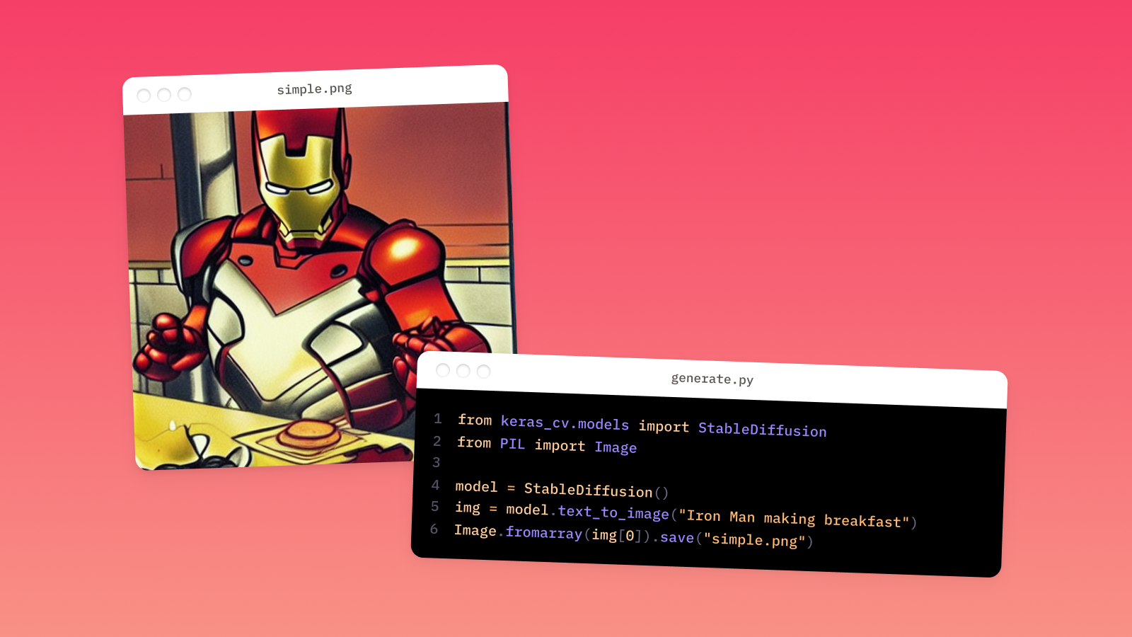
img = model.text_to_image("Iron Man making breakfast")

We first import the StabelDiffusion class from Keras and then create an instance of it, model. We then use the text_to_image() method of this model to generate an image and save it to the img variable.

If we want, in addition, to save the image, we can import and use Pillow:

from keras_cv.models import StableDiffusion
from PIL import Image

model = StableDiffusion()
img = model.text_to_image("Iron Man making breakfast")
Image.fromarray(img[0]).save("simple.png")

We select the first (and only) image from the batch as img[0] and then convert it to a Pillow Image via fromarray(). Finally, we save the image to the filepath ./simple.png via the .save() method.

With a terminal opened in the project directory, you can run the above script by entering the following command, which runs the simple.py script:

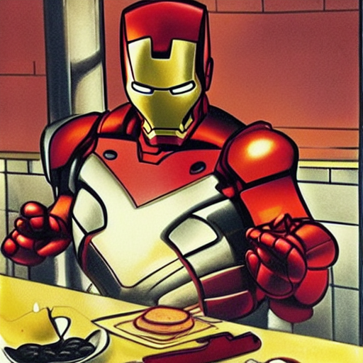
python simple.py

Again, you may need to use python3 instead of python. The following image of "Iron Man making breakfast" is generated and saved to ./simple.png:

That all it takes to use Stable Diffusion in Keras! In the next section, we'll look at more advanced usage like inpainting. Alternatively, jump down to the JIT compilation via XLA section to see how Keras can boost the speed of Stable Diffusion.

How to Use Stable Diffusion in Keras - Advanced

We'll now take a look at advanced usage, both for image generation and inpainting. The Colab notebook linked below makes it easy to e.g. modify the inpainting region with sliders, so feel free to follow along there if you wish:

All of the advanced image generation and inpainting code can be found in main.py.

Image generation

When we instantiate the Stable Diffusion model, we have the option to pass in some arguments. Below, we specify both the image height and width as 512 pixels. Each of these values must be a multiple of 128, and will be rounded to the nearest value if they are not. In addition, we also specify that we do not want to just-in-time compile the model with XLA (more details in the JIT compilation via XLA section).

model = StableDiffusion(img_height=512, img_width=512, jit_compile=False)

Next, we create a dictionary of arguments that will be passed in to the text_to_image() method. The arguments are:

• prompt - a description of the scene you would like an image of
• batch_size - the number of images to generate in an inference (constrained by memory)
• num_steps - the number of steps to use in the Diffusion process
• unconditional_guidance_scale - the guidance weight for classifier-free guidance
• seed - a random seed to use

options = dict(
    prompt="An alien riding a skateboard in space, vaporwave aesthetic, trending on ArtStation ",
    batch_size=1,
    num_steps=25,
    unconditional_guidance_scale=7,
    seed=119
)

From here, the process is very similar to above - we run the inference and then save the output as generated.png.

img = model.text_to_image(**options)
Image.fromarray(img[0]).save("generated.png")

Note that this can be done on both CPU and GPU. With an i5-11300H, it takes about 5 minutes to generate an image using the above settings. With a GPU, it should only take around 30 seconds.

Image inpainting

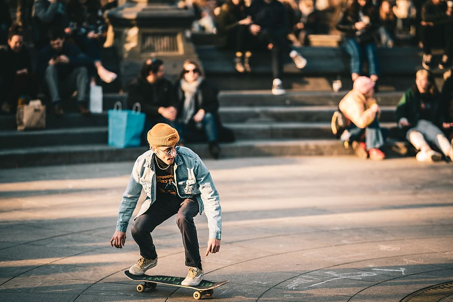
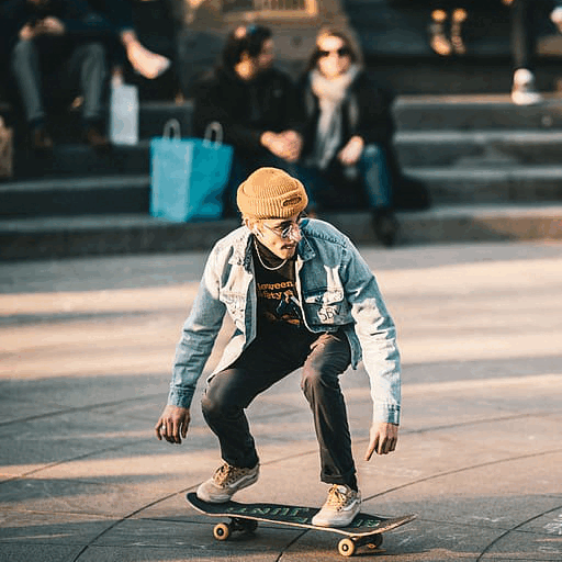
Now we'll take a look at how to inpaint using Stable Diffusion in Keras. First we download an image to modify as man-on-skateboard.jpg using the requests package:

file_URL = "https://c0.wallpaperflare.com/preview/87/385/209/man-riding-on-the-skateboard-photography.jpg"
r = requests.get(file_URL)
with open("man-on-skateboard.jpg", 'wb') as f:
    f.write(r.content)

This is the resulting downloaded image

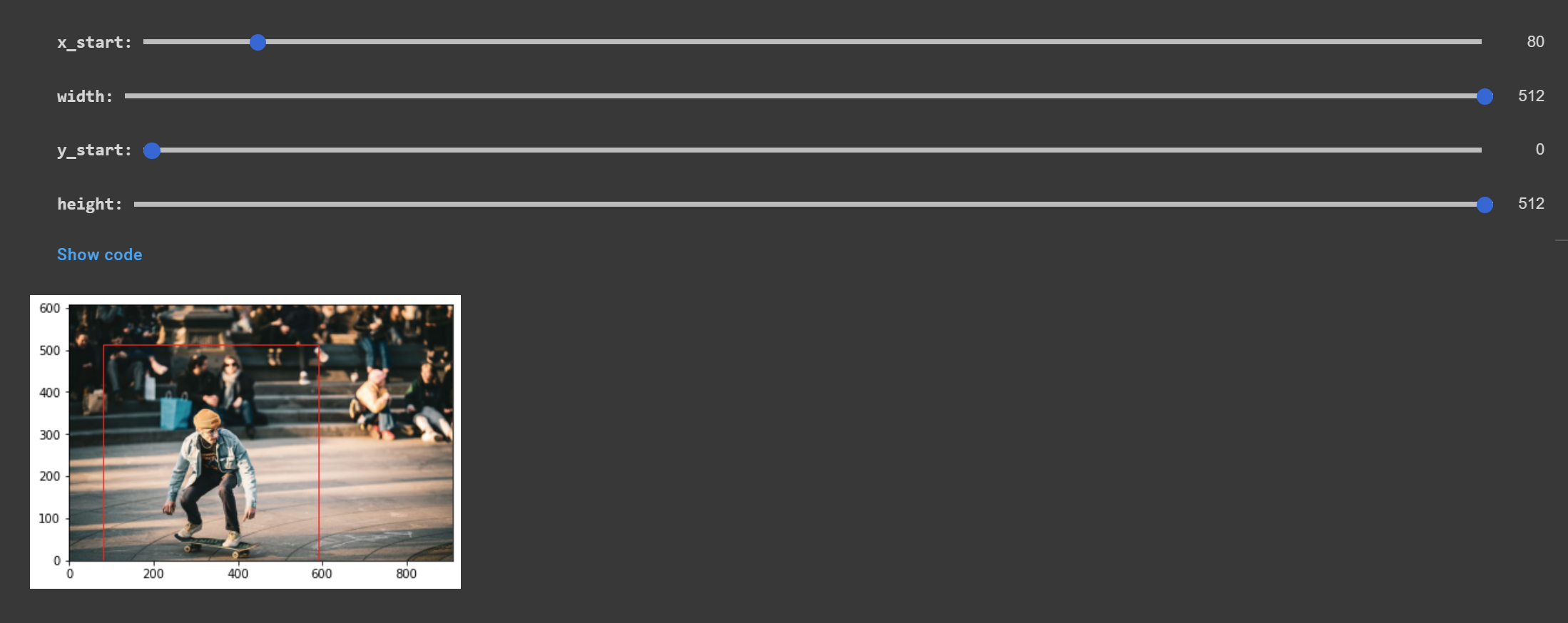
This image is 910 x 607 pixels. Before we continue, we crop it down to 512 x 512 pixels. We define the bottom left corner of the cropping region as (x_start, y_start) and set the cropping region to be 512 pixels wide and 512 pixels tall.

x_start = 80  # Starting x coordinate from the left of the image
width = 512
y_start = 0  # Starting y coordinate from the BOTTOM of the image
height = 512

If you are following along in Colab, you can use the sliders to adjust these values:

Then we open the original image and convert it to a NumPy array so that we can modify it:

im = Image.open("man-on-skateboard.jpg")
img = np.array(im)

We perform the crop, where the unusual arithmetic for the y direction stems from the fact that we defined our crop with an origin at the bottom-left of our image, while NumPy treats the top-left of the image as the origin. We then save the cropped image to man-on-skateboard-cropped.png.

img = img[im.height-height-y_start:im.height-y_start, x_start:x_start+width]
new_filename = "man-on-skateboard-cropped.png"
Image.fromarray(img).save(new_filename)

Now it's time to create the inpainting mask. The inpainting mask defines the region of the image that we want Stable Diffusion to modify. We define the values here:

x_start = 134
x_end = 374
y_start = 0
y_end = 369

Again, if you're following along in the Colab notebook, you can adjust this region with the sliders.

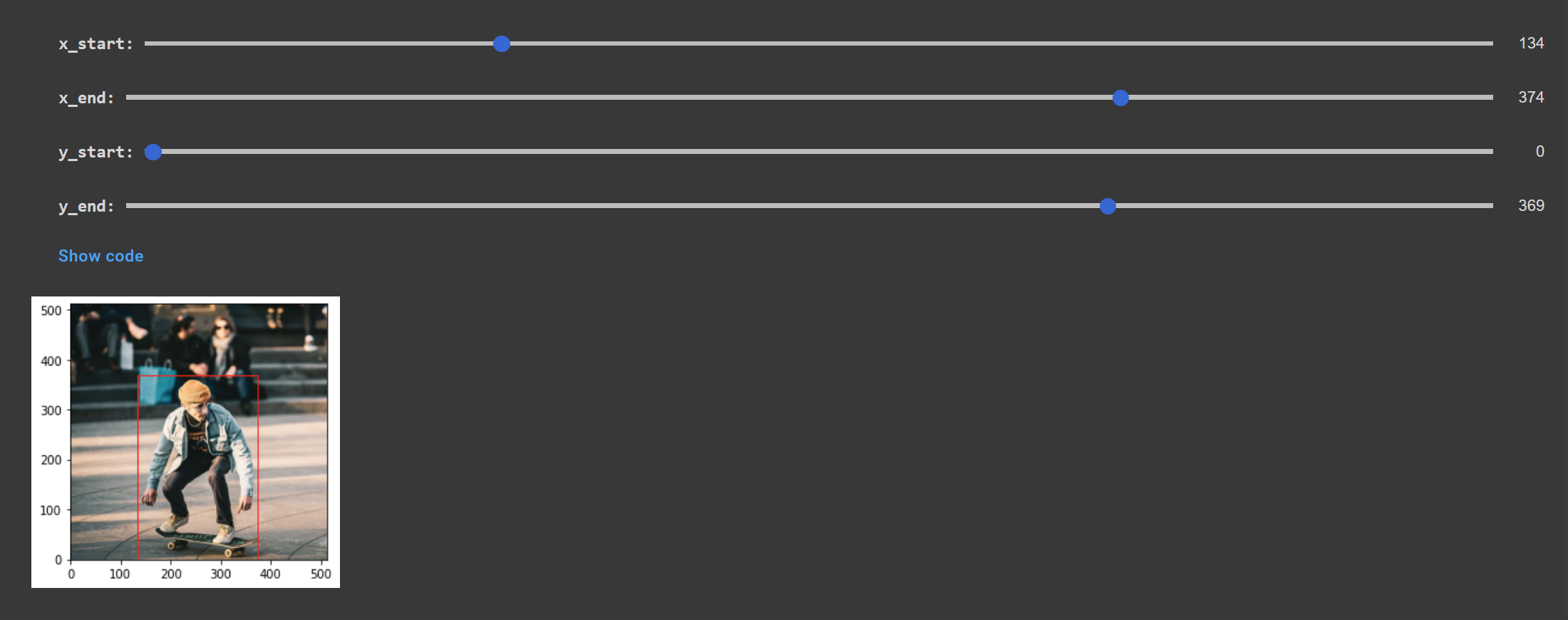
We open the cropped image as an array like before, and then create a mask with the same shape as the array, where each value in the array is a 1. We then replace the region defined by the inpainting mask with zeros, which tells the model that this is the region we want inpainted.

im = Image.open("man-on-skateboard-cropped.png")
img = np.array(im)

# Intiialize
mask = np.ones((img.shape[:2]))
# Apply mask
mask[img.shape[0]-y_start-y_end:img.shape[1]-y_start, x_start:x_end] = 0

Next, we expand the dimensions of both the mask and image arrays because the model expects a batch dimension.

mask = np.expand_dims(mask, axis=0)
img = np.expand_dims(img, axis=0)

Now its time to define our inpainting options. We pass in the image array to the img argument and the mask array to the mask argument. Besides this, all of the arguments are the same except for the following:

• num_resamples - how many times the inpainting is resampled. Increasing this number will improve semantic fit at the cost of more computation
• diffusion_noise - optional custom noise to seed the Diffusion process - either seed or diffusion_noise must be provided, but not both
• verbose - a boolean that defines whether a progress bar should be printer

inpaint_options = dict(
        prompt="A golden retriever on a skateboard",
        image=img,  # Tensor of RGB values in [0, 255]. Shape (batch_size, H, W, 3)
        mask=mask,  # Mask of binary values of 0 or 1
        num_resamples=5,
        batch_size=1,
        num_steps=25,
        unconditional_guidance_scale=8.5,
        diffusion_noise=None,
        seed=SEED,
        verbose=True,
)

Finally, we again instantiate the model, run the inference, and save the resulting array, as above. The image is saved to ./inpainted.png.

inpainting_model = StableDiffusion(img_height=img.shape[1], img_width=img.shape[2], jit_compile=False)

inpainted = inpainting_model.inpaint(**inpaint_options)

Image.fromarray(inpainted[0]).save("inpainted.png")

Below we can see a GIF of the original cropped image, the inpainting region, and the resulting image generated by Stable Diffusion.

It is again possible to run this inference on both CPU and GPU. With an i5-11300H, it takes about 22 minutes to run an inpainting using the above settings. With a GPU, it should only take a couple of minutes.

JIT compilation via XLA

Languages like C++ are traditionally ahead-of-time (AOT) compiled, meaning that the source code is compiled to machine code, and then this machine code is executed by the processor. On the other hand, Python is generally interpreted. This means that the source code is not compiled ahead of time and is instead interpreted by the processor at runtime. While no compilation step is required, interpretation is slower than running an executable.

Just-in-time (JIT) compilation is the process of compiling code at runtime. While there is some overhead in compiling the function, once it is compiled it can be executed much faster than an interpreted equivalent. This means that functions that are repeatedly called will see benefits from JIT compilation.

XLA, or accelerated linear algebra, is a domain-specific compiler built specifically for linear algebra. Stable Diffusion in Keras supports JIT compilation via XLA. That means that we can compile Stable Diffusion into an XLA-compiled version that has the potential to execute much faster than other implementations of Stable Diffusion.

Benchmarks

We see in the graph below that leveraging XLA allows Keras's implementation of Stable Diffusion to execute notably faster than the Hugging Face implementation in the diffusers library:

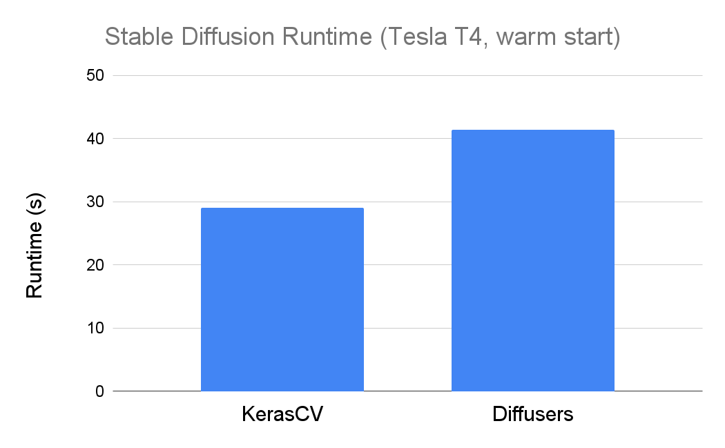
Note that these numbers reflect warm-start generation - Keras is actually slower from a cold start. This is to be expected given that the compilation step adds time to the cold-start generation. As noted here, this is not a big issue given that, in a production environment, compilation would be a one-time cost that is amortized over the (hopefully) many, many inferences that the model would run.

Combining XLA and mixed precision together allows for the fastest execution speeds. Below we see the runtimes for all combinations of with/without XLA and mixed precision:

You can run these experiments yourself on Colab here or check out some additional metrics like cold start times here.

Conclusion

That's all it takes to get started with Stable Diffusion with Keras! A highly performant implementation that requires just a few lines of code, Keras's Stable Diffusion is a great choice for a wide range of applications.

If you have more questions about text-to-image models, check out some of the below resources for further learning:

1. How do I build a text-to-image model?
2. What is classifier-free guidance?
3. What is prompt engineering?
4. How does DALL-E 2 work?
5. How does Imagen work?

Alternatively, consider following our YouTube channel, Twitter, or newsletter to stay up to date with our latest tutorials and deep dives!