What is Residual Vector Quantization?
Neural Audio Compression methods based on Residual Vector Quantization are reshaping the landscape of modern audio codecs. In this guide, learn the basic ideas behind RVQ and how it enhances Neural Compression.


Data compression plays a pivotal role in today’s digital world, facilitating efficient storage and transmission of information. As over 80% of internet traffic today is due to audio and video streaming, developing more efficient data compression can have a considerable impact – with cost reductions and significant improvements in the web's overall energy and carbon footprint.
Traditional compression algorithms have been centered on reducing redundancies in data sequences –be it in images, videos, or audio– with a high reduction in file size at the cost of some loss of information from the original. The MP3 encoding algorithm significantly changed how we store and share music data and stands as a famous example.
Neural Compression techniques are rapidly emerging as a new approach, employing neural networks to represent, compress, and reconstruct data, potentially achieving high compression rates with nearly zero perceptual information loss.
In the audio domain, in particular, neural audio codecs based on Residual Vector Quantization supersede traditionally handcrafted pipelines. State-of-the-art AI models like Google's SoundStream and EnCodec by Meta AI are already proficient in encoding audio signals across a broad spectrum of bitrates, marking a significant step forward in learnable codecs.
In this blog post, we’ll outline the main ideas behind Neural Compression and Residual Vector Quantization.
Neural Compression
Neural Compression aims to transform various data types, be it in pixel form (images), waveforms (audio), or frame sequences (video), into more compact representations, such as vectors.

The point is that this transformation is not just a straightforward reduction in size: it yields a representation of data wherein patterns are automatically identified, stored, and then used for reconstruction. Such representations are called embeddings and are used extensively in deep learning, from language models to image generators.
In the context of image compression, for example, rather than recording every pixel value, Neural Compression learns to identify critical features or visual patterns. As in autoencoders, the learned features are then used to reconstruct the image with high accuracy. Analogously, waveforms can be translated into vector formats and decoded to regenerate the sound.
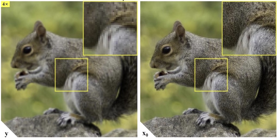
The academic discourse on Neural Compression highlights its potential for lossless or near-lossless compression capabilities, that is, the ability to compress and decompress data with minimal quality degradation. Indeed, when these models are combined with iterative denoising and diffusion for upscaling or super-resolution techniques, they can recreate data with high faithfulness to the original.

This approach gives more weight and emphasis to perceptual loss, given that human vision and auditory systems tend to notice certain details more than others. Furthermore, this technique allows the adaptive transformation of content into varying qualities (resolution, bitrate, or frame rate) based on the same vector representations.
In the next section, we look at how these general ideas are applied to compress audio data with neural audio codecs. We finally discuss a missing key component, residual vector quantization, for achieving high compression rates.
Neural Audio Codecs and RVQ
Essentially, an audio codec translates recorded sound, a digital audio signal, into a given content format. The goal is to maintain the original qualities of the sound while reducing file size and bitrate. State-of-the-art neural audio compression (or neural audio codecs) employ deep neural networks to achieve the same goal.
A simple vanilla approach based on autoencoders doesn’t help, as audio signals have a very high information density and require high-dimensional vectors to be represented correctly. Quantization techniques to reduce the dimensionality of these vectors are therefore necessary.
Let’s now take an overview of how quantization works.
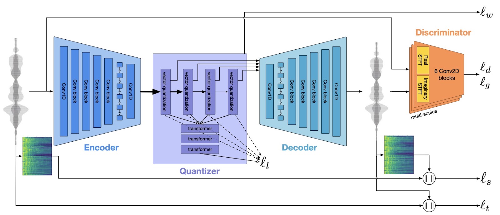
The above figure depicts the EnCodec architecture, which mirrors that of SoundStream. At its core, it's an end-to-end neural network-based approach. It consists of an encoder, a quantizer, and a decoder, all trained simultaneously.
Here's a step-by-step outline of how the pipeline operates:
- The encoder converts each fixed-length sample, just a few milliseconds of the audio waveform, into a vector of a pre-determined fixed dimensionality.
- The quantizer then compresses this encoded vector through a process known as Residual Vector Quantization, a concept originating in digital signal processing.
- Finally, the decoder takes this compressed signal and reconstructs it into an audio stream. This reconstructed audio is then compared to the original using a discriminator component. The discriminator measures the numerical difference between the two, called discriminator/generator losses.
- Besides the discriminator loss, the model calculates other types of losses. These losses include comparing the reconstructed waveform and mel-spectrogram with the original ones and assessing a commitment loss to stabilize the encoder’s output. The ultimate goal is to ensure that the audio's output closely mirrors the initial input.
The crux of the data compression occurs at the quantizer level. The following diagram illustrates the idea:

Consider an audio sample the encoder transforms into a vector of 128 dimensions.
- The first quantizer layer has a codebook table containing a fixed number of learnable vectors of the same dimension.
- The input vector is compared with those in the codebook, and the index of the most similar one is extracted.
- This is the compression stage: We've just replaced a vector of 128 numbers with a single number (the corresponding index in the codebook).
In practice, a single quantizer layer would need a very large (indeed, exponentially large) codebook to represent the compressed data accurately.
Residual Vector Quantization (RVQ) offers an elegant solution. RVQ can provide a progressively finer approximation to these high-dimensional vectors by employing a cascade of codebooks.
The idea is simple: The primary codebook offers a first-order quantization of the input vector. The residuals, or the differences between the data vectors and their quantized representations, are then further quantized using a secondary codebook.

This layered approach continues, with each stage focusing on the residuals from the previous stage, as illustrated in the figure above. Thus, rather than trying to quantize a high-dimensional vector with a single mammoth codebook directly, RVQ breaks down the problem, achieving high precision with significantly reduced computational costs.
Further Reading
To experiment with RVQ in Pytorch, you can play around with the great open-source VQ repo by lucidrains.
We recommend the recent paper High-Fidelity Audio Compression with Improved RVQGAN by R. Kumar et al. (and the literature therein) to get up to speed with the latest advances in neural audio compression. The authors introduce a high-fidelity “universal” neural audio compression algorithm that can compress all audio domains (speech, environment, music, etc.) with a single universal model, making it applicable to generative modeling of all audio. Open source code and model weights (as well as a demo page) are available.
Final Words
Neural Compression methods based on Residual Vector Quantization are revolutionizing audio (and, presumably soon, video) codecs, offering near-lossless compression capabilities while reducing computational overhead. Quantization techniques like RVQ have become essential to Text-to-Speech and Text-to-Music generators.
More broadly, innovations in neural compression signify not just an advancement in technology but also a leap towards more efficient and sustainable digital ecosystems.
Enjoyed this article? Check out our recent articles to learn about:
Lorem ipsum dolor sit amet, consectetur adipiscing elit, sed do eiusmod tempor incididunt ut labore et dolore magna aliqua. Ut enim ad minim veniam, quis nostrud exercitation ullamco laboris nisi ut aliquip ex ea commodo consequat. Duis aute irure dolor in reprehenderit in voluptate velit esse cillum dolore eu fugiat nulla pariatur.