Building an End-to-End Speech Recognition Model in PyTorch
The complete guide on how to build an end-to-end Speech Recognition model in PyTorch. Train your own CTC Deep Speech model using this tutorial.


Deep Learning has changed the game in Automatic Speech Recognition with the introduction of end-to-end models. These models take in audio, and directly output transcriptions. Two of the most popular end-to-end models today are Deep Speech by Baidu, and Listen Attend Spell (LAS) by Google. Both Deep Speech and LAS, are recurrent neural network (RNN) based architectures with different approaches to modeling speech recognition. Deep Speech uses the Connectionist Temporal Classification (CTC) loss function to predict the speech transcript. LAS uses a sequence to sequence network architecture for its predictions.
These models simplified speech recognition pipelines by taking advantage of the capacity of deep learning system to learn from large datasets. With enough data, you should, in theory, be able to build a super robust speech recognition model that can account for all the nuance in speech without having to spend a ton of time and effort hand engineering acoustic features or dealing with complex pipelines in more old-school GMM-HMM model architectures, for example.
Deep learning is a fast-moving field, and Deep Speech and LAS style architectures are already quickly becoming outdated. You can read about where the industry is moving in the Latest Advancement Section below.
#How to Build Your Own End-to-End Speech Recognition Model in PyTorch
Let's walk through how one would build their own end-to-end speech recognition model in PyTorch. The model we'll build is inspired by Deep Speech 2 (Baidu's second revision of their now-famous model) with some personal improvements to the architecture. The output of the model will be a probability matrix of characters, and we'll use that probability matrix to decode the most likely characters spoken from the audio. You can find the full code and also run the it with GPU support on Google Colaboratory.
#Preparing the data pipeline
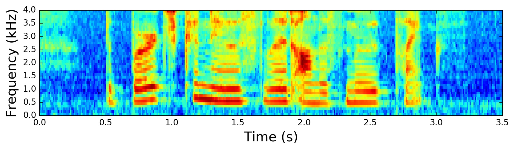
Data is one of the most important aspects of speech recognition. We'll take raw audio waves and transform them into Mel Spectrograms.
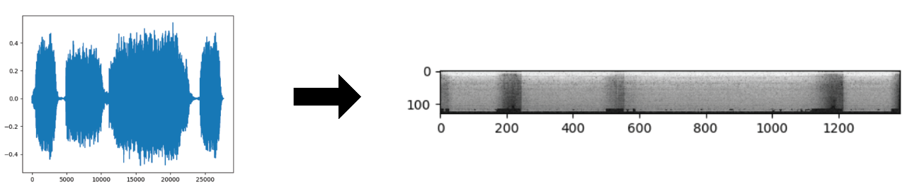
You can read more on the details about how that transformation looks from this excellent post here. For this post, you can just think of a Mel Spectrogram as essentially a picture of sound.
For handling the audio data, we are going to use an extremely useful utility called torchaudio which is a library built by the PyTorch team specifically for audio data. We'll be training on a subset of LibriSpeech, which is a corpus of read English speech data derived from audiobooks, comprising 100 hours of transcribed audio data. You can easily download this dataset using torchaudio:
import torchaudio
train_dataset = torchaudio.datasets.LIBRISPEECH("./", url="train-clean-100", download=True)
test_dataset = torchaudio.datasets.LIBRISPEECH("./", url="test-clean", download=True)
Each sample of the dataset contains the waveform, sample rate of audio, the utterance/label, and more metadata on the sample. You can view what each sample looks like from the source code here.
Experience Speech Recognition in Action
Try our API with your own audio files in our interactive playground - no coding required.
#Data Augmentation - SpecAugment
Data augmentation is a technique used to artificially increase the diversity of your dataset in order to increase your dataset size. This strategy is especially helpful when data is scarce or if your model is overfitting. For speech recognition, you can do the standard augmentation techniques, like changing the pitch, speed, injecting noise, and adding reverb to your audio data.
We found Spectrogram Augmentation (SpecAugment), to be a much simpler and more effective approach. SpecAugment, was first introduced in the paper SpecAugment: A Simple Data Augmentation Method for Automatic Speech Recognition, in which the authors found that simply cutting out random blocks of consecutive time and frequency dimensions improved the models generalization abilities significantly!
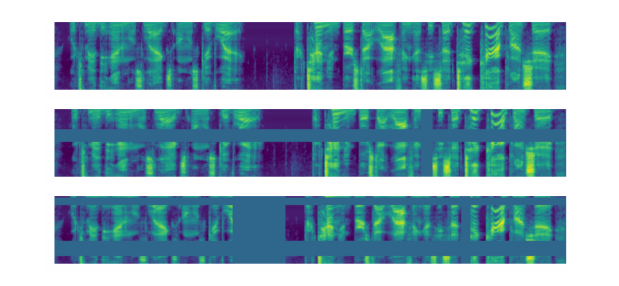
In PyTorch, you can use the torchaudio function FrequencyMasking to mask out the frequency dimension, and TimeMasking for the time dimension.
torchaudio.transforms.FrequencyMasking()
torchaudio.transforms.TimeMasking()
Now that we have the data, we'll need to transform the audio into Mel Spectrograms, and map the character labels for each audio sample into integer labels:
char_map_str = """
 ' 0
 <SPACE> 1
 a 2
 b 3
 c 4
 d 5
 e 6
 f 7
 g 8
 h 9
 i 10
 j 11
 k 12
 l 13
 m 14
 n 15
 o 16
 p 17
 q 18
 r 19
 s 20
 t 21
 u 22
 v 23
 w 24
 x 25
 y 26
 z 27
 """
class TextTransform:
"""Maps characters to integers and vice versa"""
def __init__(self):
char_map_str = char_map_str
self.char_map = {}
self.index_map = {}
for line in char_map_str.strip().split('\n'):
ch, index = line.split()
self.char_map[ch] = int(index)
self.index_map[int(index)] = ch
self.index_map[1] = ' '
def text_to_int(self, text):
""" Use a character map and convert text to an integer sequence """
int_sequence = []
for c in text:
if c == ' ':
ch = self.char_map['']
else:
ch = self.char_map[c]
int_sequence.append(ch)
return int_sequence
def int_to_text(self, labels):
""" Use a character map and convert integer labels to an text sequence """
string = []
for i in labels:
string.append(self.index_map[i])
return ''.join(string).replace('', ' ')
train_audio_transforms = nn.Sequential(
torchaudio.transforms.MelSpectrogram(sample_rate=16000, n_mels=128),
torchaudio.transforms.FrequencyMasking(freq_mask_param=15),
torchaudio.transforms.TimeMasking(time_mask_param=35)
)
valid_audio_transforms = torchaudio.transforms.MelSpectrogram()
text_transform = TextTransform()def data_processing(data, data_type="train"):
spectrograms = []
labels = []
input_lengths = []
label_lengths = []
for (waveform, _, utterance, _, _, _) in data:
if data_type == 'train':
spec = train_audio_transforms(waveform).squeeze(0).transpose(0, 1)
else:
spec = valid_audio_transforms(waveform).squeeze(0).transpose(0, 1)
spectrograms.append(spec)
label = torch.Tensor(text_transform.text_to_int(utterance.lower()))
labels.append(label)
input_lengths.append(spec.shape[0]//2)
label_lengths.append(len(label))
spectrograms = nn.utils.rnn.pad_sequence(spectrograms, batch_first=True).unsqueeze(1).transpose(2, 3)
labels = nn.utils.rnn.pad_sequence(labels, batch_first=True)
return spectrograms, labels, input_lengths, label_lengths
#Define the Model - Deep Speech 2 (but better)
Our model will be similar to the Deep Speech 2 architecture. The model will have two main neural network modules - N layers of Residual Convolutional Neural Networks (ResCNN) to learn the relevant audio features, and a set of Bidirectional Recurrent Neural Networks (BiRNN) to leverage the learned ResCNN audio features. The model is topped off with a fully connected layer used to classify characters per time step.

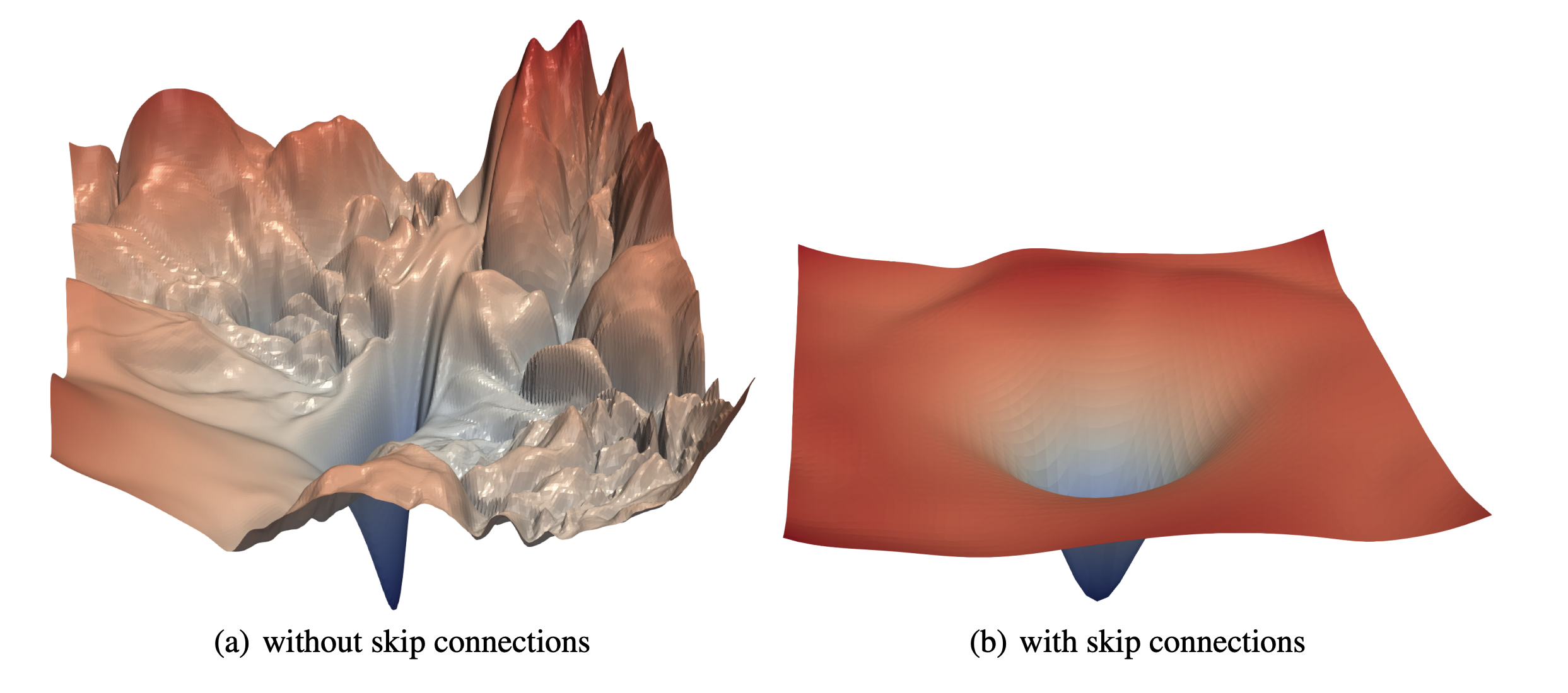
Convolutional Neural Networks (CNN) are great at extracting abstract features, and we'll apply the same feature extraction power to audio spectrograms. Instead of just vanilla CNN layers, we choose to use Residual CNN layers. Residual connections (AKA skip connections) were first introduced in the paper Deep Residual Learning for Image Recognition, where the author found that you can build really deep networks with good accuracy gains if you add these connections to your CNN's. Adding these Residual connections also helps the model learn faster and generalize better. The paper Visualizing the Loss Landscape of Neural Nets shows that networks with residual connections have a “flatter” loss surface, making it easier for models to navigate the loss landscape and find a lower and more generalizable minima.
Recurrent Neural Networks (RNN) are naturally great at sequence modeling problems. RNN's processes the audio features step by step, making a prediction for each frame while using context from previous frames. We use BiRNN's because we want the context of not only the frame before each step, but the frames after it as well. This can help the model make better predictions, as each frame in the audio will have more information before making a prediction. We use Gated Recurrent Unit (GRU's) variant of RNN's as it needs less computational resources than LSTM's, and works just as well in some cases.
The model outputs a probability matrix for characters which we'll use to feed into our decoder to extract what the model believes are the highest probability characters that were spoken.
class CNNLayerNorm(nn.Module):
"""Layer normalization built for cnns input"""
def __init__(self, n_feats):
super(CNNLayerNorm, self).__init__()
self.layer_norm = nn.LayerNorm(n_feats)
def forward(self, x):
# x (batch, channel, feature, time)
x = x.transpose(2, 3).contiguous() # (batch, channel, time, feature)
x = self.layer_norm(x)
return x.transpose(2, 3).contiguous() # (batch, channel, feature, time) class ResidualCNN(nn.Module):
"""Residual CNN inspired by https://arxiv.org/pdf/1603.05027.pdf
except with layer norm instead of batch norm
"""
def __init__(self, in_channels, out_channels, kernel, stride, dropout, n_feats):
super(ResidualCNN, self).__init__()
self.cnn1 = nn.Conv2d(in_channels, out_channels, kernel, stride, padding=kernel//2)
self.cnn2 = nn.Conv2d(out_channels, out_channels, kernel, stride, padding=kernel//2)
self.dropout1 = nn.Dropout(dropout)
self.dropout2 = nn.Dropout(dropout)
self.layer_norm1 = CNNLayerNorm(n_feats)
self.layer_norm2 = CNNLayerNorm(n_feats)
def forward(self, x):
residual = x # (batch, channel, feature, time)
        x = self.layer_norm1(x)
        x = F.gelu(x)
        x = self.dropout1(x)
        x = self.cnn1(x)
        x = self.layer_norm2(x)
        x = F.gelu(x)
        x = self.dropout2(x)
        x = self.cnn2(x)
        x += residual
return x # (batch, channel, feature, time)
class BidirectionalGRU(nn.Module):
def __init__(self, rnn_dim, hidden_size, dropout, batch_first):
super(BidirectionalGRU, self).__init__()
self.BiGRU = nn.GRU(
input_size=rnn_dim, hidden_size=hidden_size,
num_layers=1, batch_first=batch_first, bidirectional=True)
self.layer_norm = nn.LayerNorm(rnn_dim)
self.dropout = nn.Dropout(dropout)
def forward(self, x):
x = self.layer_norm(x)
x = F.gelu(x)
x, _ = self.BiGRU(x)
x = self.dropout(x)
return xclass SpeechRecognitionModel(nn.Module):
"""Speech Recognition Model Inspired by DeepSpeech 2"""
def __init__(self, n_cnn_layers, n_rnn_layers, rnn_dim, n_class, n_feats, stride=2, dropout=0.1):
super(SpeechRecognitionModel, self).__init__()
n_feats = n_feats//2
self.cnn = nn.Conv2d(1, 32, 3, stride=stride, padding=3//2) # cnn for extracting heirachal features
# n residual cnn layers with filter size of 32
        self.rescnn_layers = nn.Sequential(*[
            ResidualCNN(32, 32, kernel=3, stride=1, dropout=dropout, n_feats=n_feats)
for _ in range(n_cnn_layers)
])
self.fully_connected = nn.Linear(n_feats*32, rnn_dim)
self.birnn_layers = nn.Sequential(*[
BidirectionalGRU(rnn_dim=rnn_dim if i==0 else rnn_dim*2,
hidden_size=rnn_dim, dropout=dropout, batch_first=i==0)
for i in range(n_rnn_layers)
])
self.classifier = nn.Sequential(
nn.Linear(rnn_dim*2, rnn_dim), # birnn returns rnn_dim*2
            nn.GELU(),
            nn.Dropout(dropout),
            nn.Linear(rnn_dim, n_class)
        )
def forward(self, x):
x = self.cnn(x)
x = self.rescnn_layers(x)
sizes = x.size()
x = x.view(sizes[0], sizes[1] * sizes[2], sizes[3]) # (batch, feature, time)
x = x.transpose(1, 2) # (batch, time, feature)
        x = self.fully_connected(x)
        x = self.birnn_layers(x)
        x = self.classifier(x)
return x
#Picking the Right Optimizer and Scheduler - AdamW with Super Convergence
The optimizer and learning rate schedule plays a very important role in getting our model to converge to the best point. Picking the right optimizer and scheduler can also save you compute time, and help your model generalize better to real-world use cases. For our model, we'll be using AdamW with the One Cycle Learning Rate Scheduler. Adam is a widely used optimizer that helps your model converge more quickly, therefore, saving compute time, but has been notorious for not generalizing as well as Stochastic Gradient Descent AKA SGD.
AdamW was first introduced in Decoupled Weight Decay Regularization, and is considered a “fix” to Adam. The paper pointed out that the original Adam algorithm has a wrong implementation of weight decay, which AdamW attempts to fix. This fix helps with Adam's generalization problem.
The One Cycle Learning Rate Scheduler was first introduced in the paper Super-Convergence: Very Fast Training of Neural Networks Using Large Learning Rates. This paper shows that you can train neural networks an order of magnitude faster, while keeping their generalizable abilities, using a simple trick. You start with a low learning rate, which warms up to a large maximum learning rate, then decays linearly to the same point of where you originally started.
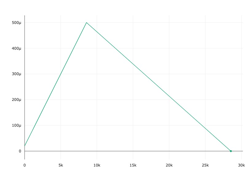
Because the maximum learning rate is magnitudes higher than the lowest, you also gain some regularization benefits which helps your model generalize better if you have a smaller set of data.
With PyTorch, these two methods are already part of the package.
optimizer = optim.AdamW(model.parameters(), hparams['learning_rate'])
scheduler = optim.lr_scheduler.OneCycleLR(optimizer,
	max_lr=hparams['learning_rate'],
steps_per_epoch=int(len(train_loader)),
epochs=hparams['epochs'],
anneal_strategy='linear')
#The CTC Loss Function - Aligning Audio to Transcript
Our model will be trained to predict the probability distribution of all characters in the alphabet for each frame (ie, timestep) in the spectrogram we feed into the model.
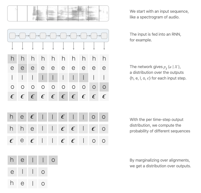
Traditional speech recognition models would require you to align the transcript text to the audio before training, and the model would be trained to predict specific labels at specific frames.
The innovation of the CTC loss function is that it allows us to skip this step. Our model will learn to align the transcript itself during training. The key to this is the “blank” label introduced by CTC, which gives the model the ability to say that a certain audio frame did not produce a character. You can see a more detailed explanation of CTC and how it works from this excellent post.
The CTC loss function is also built into PyTorch.
criterion = nn.CTCLoss(blank=28).to(device)
#Evaluating Your Speech Model
When Evaluating your speech recognition model, the industry standard is using the Word Error Rate (WER) as the metric. The Word Error Rate does exactly what it says - it takes the transcription your model outputs, and the true transcription, and measures the error between them. You can see how that's implemented here. Another useful metric is called the Character Error Rate (CER). The CER measures the error of the characters between the model's output and the true labels. These metrics are helpful to measure how well your model performs.
For this tutorial, we'll use a "greedy" decoding method to process our model's output into characters that can be combined to create the transcript. A "greedy" decoder takes in the model output, which is a softmax probability matrix of characters, and for each time step (spectrogram frame), it chooses the label with the highest probability. If the label is a blank label, we remove it from the final transcript.
def GreedyDecoder(output, labels, label_lengths, blank_label=28, collapse_repeated=True):
arg_maxes = torch.argmax(output, dim=2)
decodes = []
targets = []
for i, args in enumerate(arg_maxes):
decode = []
targets.append(text_transform.int_to_text(labels[i][:label_lengths[i]].tolist()))
for j, index in enumerate(args):
if index != blank_label:
if collapse_repeated and j != 0 and index == args[j -1]:
continue
                decode.append(index.item())
        decodes.append(text_transform.int_to_text(decode))
return decodes, targets
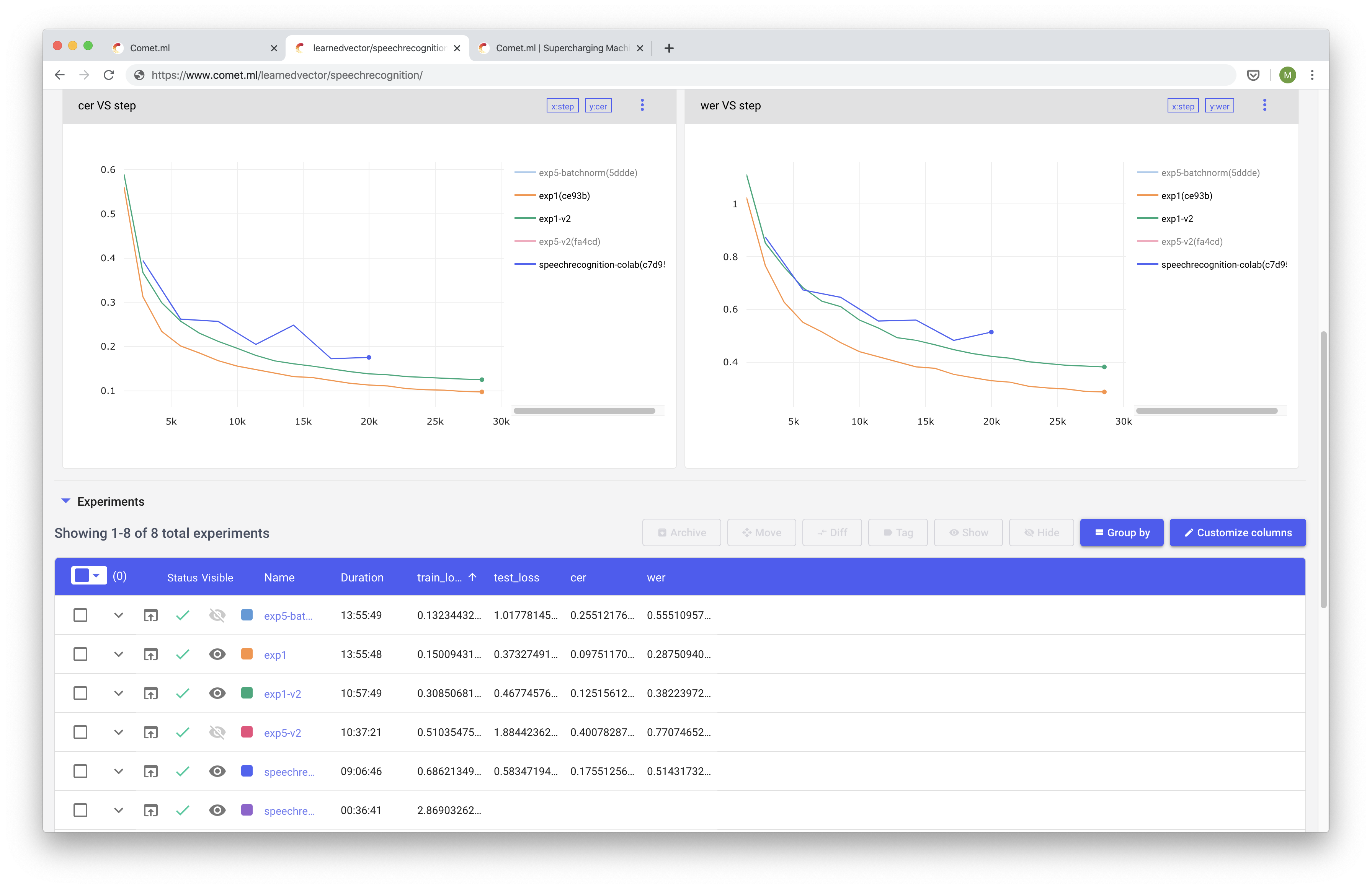
#Training and Monitoring Your Experiments Using Comet.ml
Comet.ml provides a platform that allows deep learning researchers to track, compare, explain, and optimize their experiments and models. Comet.ml has improved our productivity at AssemblyAI and we highly recommend using this platform for teams doing any sort of data science experiments. Comet.ml is super easy to set up. And works with just a few lines of code.
# initialize experiment object
experiment = Experiment(api_key=comet_api_key, project_name=project_name)
experiment.set_name(exp_name)
# track metrics
experiment.log_metric('loss', loss.item())
Comet.ml provides you with a very productive dashboard where you can view and track your model's progress.
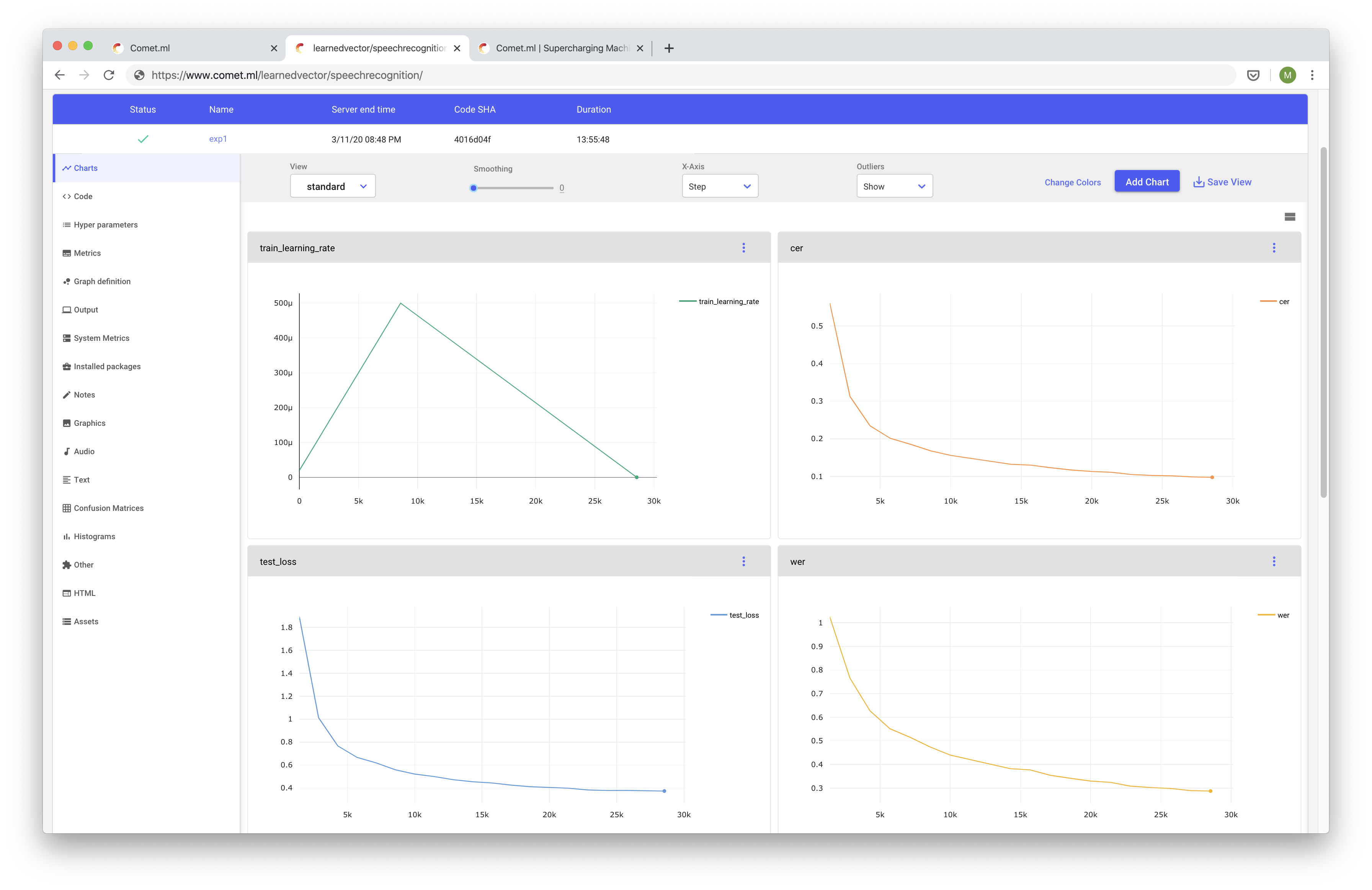
You can use Comet to track metrics, code, hyper parameters, your model's graphs, among many other things! A really handy feature that Comet provides is the ability to compare your experiment among many other experiments.
Comet has a rich feature set that we won't cover all here, but we highly recommended using it for a productivity and sanity boost. Finally, here is the rest of our training script.
class IterMeter(object):
"""keeps track of total iterations"""
def __init__(self):
self.val = 0
def step(self):
self.val += 1
def get(self):
return self.valdef train(model, device, train_loader, criterion, optimizer, scheduler, epoch, iter_meter, experiment):
model.train()
data_len = len(train_loader.dataset)
with experiment.train():
for batch_idx, _data in enumerate(train_loader):
spectrograms, labels, input_lengths, label_lengths = _data
spectrograms, labels = spectrograms.to(device), labels.to(device)
optimizer.zero_grad()
output = model(spectrograms) # (batch, time, n_class)
            output = F.log_softmax(output, dim=2)
            output = output.transpose(0, 1)
# (time, batch, n_class)
            loss = criterion(output, labels, input_lengths, label_lengths)
            loss.backward()

            experiment.log_metric('loss', loss.item(), step=iter_meter.get())
            experiment.log_metric('learning_rate', scheduler.get_lr(), step=iter_meter.get())

            optimizer.step()
            scheduler.step()
            iter_meter.step()
if batch_idx % 100 == 0 or batch_idx == data_len:
print('Train Epoch: {} [{}/{} ({:.0f}%)]\tLoss: {:.6f}'.format(
epoch, batch_idx * len(spectrograms), data_len,
100. * batch_idx / len(train_loader), loss.item()))def test(model, device, test_loader, criterion, epoch, iter_meter, experiment):
print('\nevaluating…')
model.eval()
test_loss = 0
test_cer, test_wer = [], []
with experiment.test():
with torch.no_grad():
for I, _data in enumerate(test_loader):
spectrograms, labels, input_lengths, label_lengths = _data
spectrograms, labels = spectrograms.to(device), labels.to(device)
output = model(spectrograms) # (batch, time, n_class)
                output = F.log_softmax(output, dim=2)
                output = output.transpose(0, 1)
# (time, batch, n_class)
                loss = criterion(output, labels, input_lengths, label_lengths)
test_loss += loss.item() / len(test_loader)
decoded_preds, decoded_targets = GreedyDecoder(output.transpose(0, 1), labels, label_lengths)
for j in range(len(decoded_preds)):
test_cer.append(cer(decoded_targets[j], decoded_preds[j]))
test_wer.append(wer(decoded_targets[j], decoded_preds[j]))
avg_cer = sum(test_cer)/len(test_cer)
avg_wer = sum(test_wer)/len(test_wer)
experiment.log_metric('test_loss', test_loss, step=iter_meter.get())
experiment.log_metric('cer', avg_cer, step=iter_meter.get())
experiment.log_metric('wer', avg_wer, step=iter_meter.get())
print('Test set: Average loss: {:.4f}, Average CER: {:4f} Average WER: {:.4f}\n'.format(test_loss, avg_cer, avg_wer))def main(learning_rate=5e-4, batch_size=20, epochs=10,
train_url="train-clean-100", test_url="test-clean",
experiment=Experiment(api_key='dummy_key', disabled=True)):
hparams = {
"n_cnn_layers": 3,
"n_rnn_layers": 5,
"rnn_dim": 512,
"n_class": 29,
"n_feats": 128,
"stride": 2,
"dropout": 0.1,
"learning_rate": learning_rate,
"batch_size": batch_size,
"epochs": epochs
}
experiment.log_parameters(hparams)
use_cuda = torch.cuda.is_available()
torch.manual_seed(7)
device = torch.device("cuda" if use_cuda else "cpu")
if not os.path.isdir("./data"):
os.makedirs("./data")
train_dataset = torchaudio.datasets.LIBRISPEECH("./data", url=train_url, download=True)
test_dataset = torchaudio.datasets.LIBRISPEECH("./data", url=test_url, download=True)
kwargs = {'num_workers': 1, 'pin_memory': True} if use_cuda else {}
train_loader = data.DataLoader(dataset=train_dataset,
batch_size=hparams['batch_size'],
shuffle=True,
collate_fn=lambda x: data_processing(x, 'train'),
**kwargs)
test_loader = data.DataLoader(dataset=test_dataset,
batch_size=hparams['batch_size'],
shuffle=False,
collate_fn=lambda x: data_processing(x, 'valid'),
**kwargs)
model = SpeechRecognitionModel(
hparams['n_cnn_layers'], hparams['n_rnn_layers'], hparams['rnn_dim'],
hparams['n_class'], hparams['n_feats'], hparams['stride'], hparams['dropout']
).to(device)
print(model)
print('Num Model Parameters', sum([param.nelement() for param in model.parameters()]))
optimizer = optim.AdamW(model.parameters(), hparams['learning_rate'])
criterion = nn.CTCLoss(blank=28).to(device)
scheduler = optim.lr_scheduler.OneCycleLR(optimizer, max_lr=hparams['learning_rate'],
steps_per_epoch=int(len(train_loader)),
epochs=hparams['epochs'],
anneal_strategy='linear')
iter_meter = IterMeter()
for epoch in range(1, epochs + 1):
train(model, device, train_loader, criterion, optimizer, scheduler, epoch, iter_meter, experiment)
test(model, device, test_loader, criterion, epoch, iter_meter, experiment)
The train function trains the model on a full epoch of data. The test function evaluates the model on test data after every epoch. It gets the test_loss as well as the cer and wer of the model. You can start running the training script right now with GPU support in the Google Colaboratory.
#How to Improve Accuracy
Speech Recognition Requires a ton of data and a ton of compute resources. The example laid out is trained on a subset of LibriSpeech (100 hours of audio) and a single GPU. To get state of the art results you'll need to do distributed training on thousands of hours of data, on tens of GPU's spread out across many machines.
Another way to get a big accuracy improvement is to decode the CTC probability matrix using a Language Model and the CTC beam search algorithm. CTC type models are very dependent on this decoding process to get good results. Luckily there is a handy open source library that allows you to do that.
This tutorial was made to be more accessible so it's a relatively small model (23 million Parameters) compared to something like BERT (340 million Parameters). It seems to be the larger you can get your network, the better it performs, although there are diminishing returns. A larger model equating to better performance is not always the case though, as proven by OpenAI's research Deep Double Descent.
This model has 3 residual CNN layers and 5 Bidirectional GRU layers which should allow you to train a reasonable batch size on a single GPU with at least 11GB of memory. You can tweak some of the hyper parameters in the main function to reduce or increase the model size for your use case and compute availability.
#Latest Advancements In Speech Recognition with Deep Learning
Deep learning is a fast-moving field. It seems like you can't go a week without some new technique getting state of the art results. Here are a few of things worth exploring int the world of speech recognition.
Transformers
Transformers have taken the Natural Language Processing world by storm! First Introduced in the paper Attention Is All You Need, transformers have been taking and modified to beat pretty much all existing NLP task dethroning RNN's type architectures. The Transformer's ability to see the full context of sequence data is transferable to speech as well.
Unsupervised Pre-training
If you follow deep learning closely you've probably heard of BERT, GPT, and GPT2. These Transformer models have first pertained on a language modeling task with unlabeled text data, and fine-tuned on a wide array of NLP task and get state of the art results! During pre-training, the model learns something fundamental on the statistics of language and uses that power to excel at other tasks. We believe this technique has great promises on speech data as well.
Word Piece Models
Our model defined above output characters. Some benefits to that are the model doesn't have to worry about out of vocabulary words when running inference on speech. So for the word c h a t each character has is its own label. The downside to using characters are inefficiency and the model being prone to more errors because you're predicting one character at a time. Using the whole word as labels have been explored, to some degree of success. Using this method, the entire word chat would be the label. But using whole words, you would have to keep an index of all possible vocabularies to make a prediction, which is memory inefficient with the possibility of running into out of vocabulary words during prediction. The sweet spot would be using word piece or sub-word units as labels. Instead of characters for the individual label, you can chop up the words into sub-word units, and use those as labels, i.e. ch at. This solves the out of vocabulary issue, and is much more efficient, as it needs fewer steps to decode then using characters, and without the need to have an index of all possible words. Word pieces have been used successfully with many NLP models, like BERT and would work natural with speech recognition problems as well.
Lorem ipsum dolor sit amet, consectetur adipiscing elit, sed do eiusmod tempor incididunt ut labore et dolore magna aliqua. Ut enim ad minim veniam, quis nostrud exercitation ullamco laboris nisi ut aliquip ex ea commodo consequat. Duis aute irure dolor in reprehenderit in voluptate velit esse cillum dolore eu fugiat nulla pariatur.
Related posts