An Introduction to Poisson Flow Generative Models
Poisson Flow Generative Models (PFGMs) are a new type of generative Deep Learning model, taking inspiration from physics much like Diffusion Models. Learn the theory behind PFGMs and how to generate images with them in this easy-to-follow guide.


Generative AI models have made great strides in the past few years. Physics-inspired Diffusion Models have ascended to state-of-the-art performance in several domains, powering models like Stable Diffusion, DALL-E 2, and Imagen.
Researchers from MIT have recently unveiled a new physics-inspired generative model, this time drawing inspiration from the field of electrostatics. This new type of model - the Poisson Flow Generative Model (PFGM) - treats the data points as charged particles. By following the electric field generated by the data points, PFGMs can create entirely novel data.
PFGMs constitute an exciting foundation for new avenues of research, especially given that they are 10-20 times faster than Diffusion Models on image generation tasks, with comparable performance.
In this article, we'll take a high-level look at PFGM theory before learning how to train and sample with PFGMs. After that we'll take another look at the theory, this time perfoming a deep dive starting from first principles. Then we'll look at how PFGMs stack up to other models and other results before ending with some final words. For a less technical, more intuitive explanation of PFGMs, check out our How physics advanced Generative AI article. Let's dive in!
#Introduction
Several families of generative models have evolved throughout the development of AI. Some approaches, like Normalizing Flows, offer explicit estimates of sample likelihoods. Other approaches, like GANs, cannot explicitly calculate likelihoods, but can generate very high-quality samples.
Over the past couple of years, significant research efforts have been undertaken to develop Diffusion Models. Diffusion Models draw inspiration from physics, in particular thermodynamics/statistical physics, noting that e.g. any localized distribution of a gas will eventually spread out to fill an entire space evenly simply through random motion.
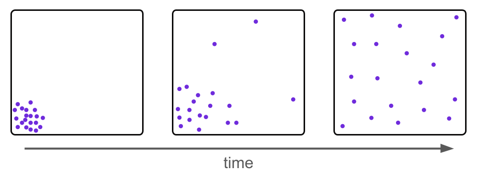
That is, any starting distribution is transformed into a uniform distribution over time. Diffusion Models draw inspiration from this idea and place e.g. images in a "high dimensional room", corrupting them with random noise in a similar way.

The goal is to train a Machine Learning model that learns how to go backwards through time, reversing this corruption process. If we can successfully learn such a mapping, then we have a transformation from a simple distribution (Gaussian, in the case of Diffusion Models) to the data distribution. We can then generate data simply by sampling from a Gaussian distribution and applying the learned transformation.
Poisson Flow Generative Models are inspired in a very similar manner to Diffusion Models, but they pull from the field of electrostatics rather than thermodynamics. The fundamental and foundational finding is that any distribution of electrons in a hyperplane generates an electric field that transforms the distribution into a uniform angular distribution as the distribution evolves through time according to the dynamics defined by the field.

If we know the electric field (aka Poisson field) generated by a distribution, then we can start with points uniformly sampled on a hemisphere and run the dynamics in reverse time to recover the original data distribution. The laws of physics, therefore, provide an invertible mapping between a simple distribution and the data distribution, yielding a means to generate novel data akin to normalizing flows.
With the overarching working principle of PFGMs in our minds, let's now take a closer look at how this working principle manifests in practice.
#Poisson Flow Generative Models - Overview
As mentioned above, the performance of PFGMs hinges on the result that the Poisson field generated by (almost) any distribution in a hyperplane results in a uniform angular distribution at a far enough distance. Intuitively, let's consider why this is the case.
Consider the electric field generated by an arbitrary charge distribution. Very close to the distribution, the electric field will be very complicated and, in general, have high curvature.

However, at a very far distance d from the charge distribution, the field is much simpler. At such a distance, all points in the charge distribution are roughly the same distance away from d. This means that the charge distribution can be considered to "collapse" down to a point, concentrating all of its charge on that one point. The electric field for a point charge is quite simple - being radial in direction and inversely square to the distance from the point in magnitude:

Therefore, as we "zoom out" from the charge distribution, it looks more and more like a point charge with the corresponding electric field:

In general, physical fields are well-behaved, and the electromagnetic field is no exception. Therefore, the locally complicated electric field near the distribution (or source), must connect in a smooth way to the electric field far from the distribution, which we have seen to be purely radial, so the electric field lines will look something like this:

Given that the electric field is radial at a very far distance, the surface tangential to the field is spherical at this distance. The PFGM authors prove that, not only is this surface spherical, but its flux density is uniform. Below we see a heart-shaped charge distribution in the z=0 plane along with some of the electric field lines (black arrows) it generates. The flux density through the enclosing hemispherical surface is (nearly) uniform.
Proof Intuition

As a result, if we let the charge distribution evolve along the field lines, it will transform into a uniform hemispherical distribution.

If we learn the Poisson field in a high-dimensional space for e.g. an image data distribution, then we can simply sample points uniformly from the high-dimensional hemisphere and run the dynamics in reverse time to generate images from the data distribution:

How do we go about learning and using the Poisson field generated by a data distribution?
Learning the Poisson field
We seek to model the dynamics of particles under the influence of the Poisson field generated by a data distribution. Let's take a look at how we learn this Poisson field now.
Terminology Note
Step 1 - Augment the data
Below we see a video of a distribution that spells "PFGM" evolving according to the Poisson field it generates. In particular, we note that the data distribution lies in a 2-dimensional plane but is mapped onto a 3-dimensional hemisphere
This is true in general with PFGMs - N-dimensional data are augmented with an additional dimension z and placed in the z=0 hyperplane of the new (N+1)-dimensional space. The data are then mapped to an (N+1)-dimensional hemisphere.
The reason for this spatial augmentation is to avoid mode collapse. Below we see the (negative) Poisson field generated by a uniform disk in the XY plane. Our sampling process involves randomly selecting points in space and following the field back to the data distribution. As we can see, all trajectories converge to the origin, meaning that our model will generate images that have no variety and therefore suffer from mode collapse.

Augmenting the data with an additional dimension circumvents this issue. Below we see the same 2-dimensional uniform disk from above now in the XY plane with the augmented dimension Z.

While we still have an intrinsically 2-dimensional data distribution, it is now embedded in a 3-dimensional space, thus generating a 3-dimensional Poisson field. If we now sample points in this 3-dimensional space, for example from the YZ plane, and follow their trajectories through the field to the XY, we are afforded a range of new trajectories that no longer collapse to the origin and instead intersect different points in the data distribution. That is, our model no longer suffers from mode collapse.
Step 2 - Calculate the empirical field
To sample with PFGMs, we must know the Poisson field. To learn the Poisson field exactly, we would need to know the data distribution exactly, but the data distribution is what we seek to sample from. If we already knew the distribution's analytical form in the first place, we would not care about the Poisson field it generates.
Rather than attempt to learn the exact Poisson field, we will instead learn the empirical field that is generated by the training data treated as point charges. Some readers may notice that this approach is reminiscent of the kinematics problem in our introduction to Differentiable Programming.
Differentiable Programming - A Simple Introduction
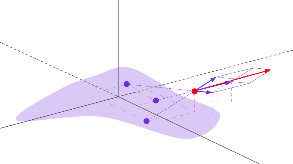
Below is an example distribution (light purple) which we seek to generate data for, along with several data points sampled from this distribution (purple points). In addition, there is a randomly selected point in space (red point) at which we seek to estimate the Poisson field (or, equivalently, calculate the empirical field).

To calculate the empirical electric field, we sum the field generated by each data point-charge, which is equivalent to the total empirical field at this point due to the superposition principle. Each individual data point's field contribution can be seen below as a purple arrow, along with the net field represented by a red arrow.
We calculate the empirical field for many randomly sampled points in the space, with a sampling preference for points close to the data points since the curvature of the field will be more dramatic in these regions, therefore requiring greater resolution to sufficiently approximate.
Step 3 - Calculate the loss and update the function approximator
In order to sample with PFGMs, we require a continuous analytical representation of the Poisson field, not values only at discrete points like those we calculated above. We therefore must train a function approximator for the empirical field on these points. What should this approximator look like?
The function approximator must accept an N+1 dimensional vector, representing a point in our augmented space, and return and N+1 dimensional vector, representing the empirical field at that point. The natural choice for such a mapping is a U-Net architecture, which the PFGM authors implement.

To train the U-Net, we simply calculate the average L2 loss over the batch, and then train with a gradient-based optimizer like Adam. That's it!
Sampling with PFGMs
In the last section, we learned how to train a function approximator for the empirical field generated by many data points treated as charged particles. After the field estimator has been trained, how do we actually use this estimator to sample from the original data distribution?
Recall that trajectories of the Poisson field constitute a bijection between the data distribution and a uniform hemisphere. Therefore, to sample data points from the data distribution, we sample points from a uniform angular distribution, and then make them travel backwards along the Poisson field until we reach the z=0 hyperplane in which the data distribution sits. The corresponding differential equation is:

This equation says that, at each moment in time, the point should be displaced in the direction of the negative Poisson field. Therefore, the corresponding solution will be a trajectory that traces backwards along the Poisson field to the z=0 data distribution hyperplane.
In practice, to generate data using a Poisson Field Generative Model, we:
- Uniformly sample data on a large hemisphere
- Use an ODE solver to evolve the points backwards along the Poisson field
- Evolve backwards until we reach z=0, at which point we have generated novel data from the training distribution
Implementation note
That's it! Below we can see particles moving forward and backwards along the Poisson field for the heart-shaped distribution we saw above.

In the visual space, the backwards evolution in the sampling process looks like the following:

Now that we understand how PFGMs work, let's take a look at how we can use them to generate images. Alternatively, you can jump down to the Deep Dive section for a more in-depth treatment.
#Generating images with PFGMs
To learn how to generate images with PFGMs, follow the below Colab notebook.
Poisson Flow Generative Models in Colab
The notebook shows how to set up the local environment for Colab, how to download the available pre-trained models, and how to use them to sample images from CIFAR-10, CelebA (62 x 64), and the LSUN bedroom datasets.
Want to learn more about JAX?
The PFGM repository requires the installation of JAX - learn everything you need to know about JAX in our easy-to-follow overview.
Move on to the next section for a deeper look at the theory of PFGMs, or jump down to the results to see how PFGMs perform.
#Poisson Flow Generative Models - A deep dive
In this section we'll perform a more in-depth treatment of PFGMs in order to elucidate their inner workings, starting from first principles. We begin with a discussion of Gauss's Law.
Gauss's Law and potential functions
In PFGMs we seek to sample from a data distribution by casting it as a charge distribution and leveraging the dynamics defined by the electric field it produces. The relationship between a charge distribution and the field it generates is defined by Gauss's Law, as seen below (omitting constants), where E is bolded to indicate that it is a vector field.

We define a potential function to be any function whose negative gradient is the electric field. That is, phi is a potential function for E if

While potential functions have many applications, in our case we are interested in casting Gauss's Law in terms of potential functions.
The Poisson Equation and Green's Functions
Let's use the definition of the potential to plug it in to Gauss's Law:

The result, called Poisson's equation, is an equation that defines the relationship between a potential function and the charge density function that generates it. Poisson's equation is not relegated to electrodynamics and permeates many areas of physics and engineering. What is so special about this equivalent form of Gauss's Law?
If we look more closely at the structure, we see three parts. An operator (L), a scalar function (y) on which the operator acts, and another scalar function (f) that is the result of this operation.

In particular, the del-squared operator is called the LaPlacian and is a linear differential operator. That is, the application of the LaPlacian results in a linear differential equation. The problem of recovering y given L and f is a very common problem in physics and engineering.
How might we go about solving this problem? That is, for a given charge distribution how do we find a potential function it generates? To do this, we'll exploit the linearity of the operator. Let's try chopping our charge distribution up into a few small pieces as an approximation, using a finite, uniform distribution with unit height as an example.

We'll approximate this continuous distribution with point charges, using 4 in this case.

The point charges are represented by Dirac delta functions. For those unfamiliar, the Dirac delta function (or simply "delta") represents the charge density for a point charge such that integration over the function is equal to a unit charge. By this approximation, we have

How does this approximation help? Recall that the LaPlacian is a linear differential operator - we will exploit this linearity now. In particular, let's call the potential function for the i-th point charge φi. Then we have

where the last equality is valid as a result of the linearity of the LaPlacian. Therefore, we have (for a given set of boundary conditions)

We have found that we can approximate the potential by summing the potentials of point charges - an incredibly useful result that stems directly from the linearity of the LaPlacian.
Below we have plotted the potentials for each of the above point charges (the form of which we will derive later), along with the estimated potential at a point x'. We obtain this estimate by summing the values of each of the individual potentials at that point, where each contribution can be seen in the graph with the same color as the relevant potential

We can express this more succinctly - define φ′as the solution to the below equation:

That is, given a location in space i, φ′gives the potential at any point in space x generated by a Dirac delta charge distribution centered at i. Using this newly defined function, let's improve our estimate of the true potential generated by the continuous charge distribution by increasing the number of point charges we are using to approximate the distribution. For any set of points I in the space, we have

That is, the potential has been approximated as the sum of an arbitrary number of point-charge potentials which are centered at the points in I. Let's now drive the number of points up to infinity, transforming the discrete sum into an integral:

In this case, our approximation is no longer an approximation and is exactly true (if we integrate only over the regions of nonzero charge density), but there is one caveat. Recall that our delta function represents the charge density for a unit point charge. Therefore, in the integral above, we have implicitly assumed that we have a unit charge density. This works fine for our example charge density above, but what if we had a different charge density, like this:

We now have to account for the varying charge density in this distribution. In this case, we simply multiply by the charge density in the integral, scaling the unit charge density at each point by the charge distribution to give the proper value when integrated over. We also replace φ′with the symbol G to get the final form of our integral:

This is a very important result. It says that, to solve Poisson's equation for an arbitrary charge density to calculate its potential, which might require solving a very complicated differential equation, it suffices to simply solve Poisson's equation for a point charge. With only this solution and the above equation, we can, in principle, calculate the exact potential for any charge distribution. The function G above is known as Green's function, and each linear differential operator has a corresponding Green's function (aka impulse response) that is precisely the function that yields a delta function when acted upon by the operator.
So, to summarize, to find the exact potential for any charge distribution, all we have to do is find the potential for a point charge and we can, in principle, calculate the exact potential for any charge distribution.
LaPlacian Green's Function and Electric Field
As we noted above, each linear differential operator has its own Green's function. The Green's function for the LaPlacian is

Where N is the dimensionality of the space, and S is the surface area of the (N-1)-sphere with unit radius.
Our goal with PFGMs; however, is to learn the Poisson field, not the potential function. Our intuition may tell us that the above argument, i.e. that a potential function can be considered as a sum of point-charge potentials, holds for Poisson fields as well. This intuition is indeed correct, which we can see mathematically as follows

Where the x subscript indicates that the gradient is to be taken with respect to x and therefore commutes with the integral without issue. That is, it is valid to estimate the Poisson field as a sum of Poisson fields generated by point charges.
In our case, the gradient for our Green's function (i.e. the Poisson field generated by a point charge) is

Proof
Assuming that we can exploit this fact to estimate the Poisson field, how do we then use the field to generate data?
PFGM Particle Dynamics
From physics, we know the relationship between force F and momentum p:

Assuming that mass is not a time-varying quantity, we arrive at the more common formulation, where m is mass and v is velocity:

Independently, the force F on a particle with charge q in an electric field E is given by

Therefore, we might be tempted to define the dynamics in the canonical Newtonian way:

where we have set the charge and mass to unity. However, we need to travel along electric field lines in order to properly transform our data distribution into a uniform angular distribution. That is, we must remove inertia from the picture. Inertia is an object's tendency to avoid a change in motion under the influence of an external force, so in the absence of inertia particles will move along force field lines.
Intuition
Therefore, we set the Poisson field to be equal not to the time derivative of velocity, but the time derivative of displacement.

That is, instead of setting the field equal to the second derivative of displacement with respect to time, we use the first derivative. This will cause our particles to exactly follow the field lines and is a mathematical relationship that holds for any vector field in general. From a physical perspective, this situation corresponds to so called damped motion and is akin to the particles traveling under the force of the Poisson field through a viscous fluid.
PFGM - Flow Model Interpretation
Given that the particle dynamics are completely defined by this deterministic process, to map from an arbitrary, compact distribution in the z=0 hyperplane to a uniform angular distribution, we need only to calculate (or estimate) the Poisson field which the distribution generates. It's now time to revisit from a practical standpoint our above theoretical result about estimating the Poisson field from a set of point charges.
Estimating the Poisson Field
As mentioned previously, the PFGM approach of mapping N-dimensional data to an N-dimensional hemisphere suffers from mode collapse in the sampling process. Instead, the authors introduce an additional dimension z, embedding the data on the z=0 hyperplane of the N+1 dimensional space. The data distribution in the augmented space is therefore

Where we have multiplied the original data distribution by the Dirac delta function. We calculate the empirical field generated by this distribution by summing the fields generated by each data point treated as a point charge:

This equation is valid due to the linearity of the LaPlacian as we saw above. The field is scaled by c is a multiplier for numerical stability, which is perfectly valid and only modifies the dynamics by a rescaling in time.
Since the particles follow the Poisson field lines, we actually do not care about the magnitude of the field at any point on these lines (only the direction). Therefore, we normalize the field in order to convert it to a form that is more conducive to neural learning. We define the negative normalized field as

where we add the negative sign so that the field points back towards the data distribution. The negative normalized field is what our neural network will learn.
We randomly sample many points in space so we can calculate the loss between the true empirical field and our neural network's prediction. We simply perturb the data points. Given that the curvature of the Poisson field will be higher near the data distribution than far away, sampling preference is given to points in space that are closer to the data distribution so that our function approximator more closely matches the empirical field in this region. The PFGM authors choose the following method of sampling training points:

Where

Colloquially, we create training data points by perturbing the data points in random directions, sampling the distance of the perturbance from a Chi distribution (norm of the Gaussian), always ensuring that the perturbation in the z direction is positive. Tau is a hyperparameter that provides a tradeoff between learning the structure near the data distribution vs. farther away - the greater the value of tau the greater the probability of sampling a point far from the data distribution. M defines the maximum distance from the data distribution we care about modeling, sampled uniformly from [0, 300] in the PFGM paper.
The pseudocode for this process can be seen below:

As mentioned above, we use a U-Net for the neural network. It takes in an N+1 dimensional point in space and returns the predicted N+1 dimensional negative normalized field at that point. The loss is simply the average L2 loss over the batch, and gradient-based optimization is used to train the model.
Now that we have a way to train a function approximator for the empirical field, how do we use it to generate data?
Anchoring the Backwards ODE
Recall from above the forward ODE that defines the forward dynamics:
We use the following backward ODE for sampling:

Note on signs
Where it is defined on the augmented space and the true Poisson field E is replaced with the negative normalized empirical field v. Now that we have the ODE defining our backward dynamics (and therefore sampling process), we might be tempted to consider the problem solved - simply plug the ODE into an ODE solver to generate data.
The problem is that we do not know the starting and ending times of each trajectory. That is, each particle starts on a large hemisphere and evolves via the backward ODE to the data distribution in the z=0 plane, but we do not know how long this process takes. To circumvent this issue, we anchor the ODE to the physically meaningful variable z as seen below, where the subscripts of v indicate components of the field.

Now that the ODE is cast in terms of z, we know that the termination point for each particle is when it reaches the z=0 hyperplane where the data distribution lies. What are the starting points for the particles?
Determining the prior distribution
It is easy enough to sample uniformly on a hemisphere and use the resulting z components as a starting point for the ODE, but there is a slight issue. Many ODE solvers require the entire batch to have the same initial value. Points that lie on the hemisphere have many different z values, so this presents a small hurdle.
To circumvent this issue, the uniform distribution on the hemisphere is projected to the hyperplane that coincides with the top of the hemisphere, zmax. The projection is a simple radial one given that the Poisson field is purely radial as x approaches infinity. We can see a schematic in 2D below, where the red lines connect purple points on the sphere to their projection points on the green line.

This transformation constitutes a homeomorphism between the hyperplane and the hemisphere - below we can see the homeomorphism in action in three dimensions:
Radial projection of a 3-dimensional hemisphere
From this projection, we derive the prior distribution on the hyperplane, which tells us how to sample from the zmax hyperplane in a way that is equivalent to sampling from the hemisphere uniformly:

Sampling from the data distribution
We now have all of the pieces in place that we need to generate samples from the data distribution with our PFGM. First, we sample a population of particles from the prior distribution defined above. Since the distribution is rotationally symmetric, it suffices to uniformly sample norms from the below distribution

and then uniformly sample angles from 0 to 2π. The authors then perform a change of variables to achieve exponential decay in the z dimension, replacing z with t' according to

This is solved by

Trajectory endpoints
This change of variables empirically leads to 2x faster sampling with no harm to sample quality. Further, it makes sense intuitive sense - it is sensible to take smaller step sizes near the z=0 hyperplane in order to better navigate the more complicated Poisson field that exists near the data distribution.
The corresponding backward ODE after this change of variables is

Where again v is the negative normalized empirical field, for which we use our U-Net as an approximation. From here, an ODE solver is used to solve the ODE via methods like RK45 or the Euler method.
Summary
We summarize both the theoretical logic and practical details of PFGMs below:
- We have a continuous, compact data distribution in the z=0 hyperplane.
- When treated as a charge distribution, the distribution generates a Poisson field that has uniform angular flux density approaching infinity.
- The Poisson field is generated uniquely by the data distribution (given well-behaved boundary conditions). Therefore, following field lines back to the z=0 hyperplane gives us a way to sample from the data distribution.
- The forward ODE that corresponds to following field lines is obtained simply from setting the time derivative of displacement equal to the Poisson field. Therefore, the Poisson field is the only missing piece we need to sample from the data distribution.
- While we cannot get an exact analytical form of the Poisson field, we can estimate the Poisson field given a set of data points sampled from the data distribution. The Poisson field is approximately the sum of the fields generated by each data point treated as a point charge, justified by virtue of the LaPlacian being a linear differential operator. We call this approximation the empirical field.
- We seek to train a neural network to learn the empirical field.
- We randomly sample points in space, giving preference to points near the data distribution because the Poisson field is more complicated there. At each point, we calculate the true empirical field, where the Poisson field of a point charge is obtained by taking the negative gradient of the Green's function for the LaPlacian. We also calculate the neural network's predictions at the sampled points.
- We calculate the loss as the average L2 loss between the true and predicted normalized empirical fields over the sampled points. This loss is used with gradient-based optimization to train the neural network, which in this case is a U-Net (DDPM++ backbone).
- After training the neural network, we use an ODE solver to evolve a uniform population of particles on a large hemisphere (sampled equivalently from the prior distribution) backward along the Poisson field until we reach the data distribution's hyperplane, generating samples from the distribution.
#Results
The early results of PFGMs are impressive and promising. Some highlights from applying PFGMs to the task of image generation are listed below:
- PFGMs attain the best Inception scores (9.68) and best FID scores (2.35) among normalizing flow models for CIFAR-10.
- PFGMs enjoy a 10-20x faster inference speed than SDE methods that utilize similar architectures, while retaining comparable sample quality.
- The backward ODE if PFGM accommodates many different architectures.
- PFGMs demonstrate scalability to higher resolution image generation
A table of results on CIFAR-10 can be seen below, comparing PFGMs to a variety of other methods:

PFGM architecture robustness
The authors attain the best results using the DDPM++ architecture, which is a modified version of the U-Net architecture used in early Diffusion Models. However, the authors note that the PFGM approach is robust to the usage of different architectures. For example, the variance-preserving (VP) and sub-variance-preserving (sub-VP) ODEs and SDEs used in Song et. al.'s work on score-based models demonstrate strong performance using a DDPM++ backbone, but suffer with a NCSNv2 architecture, with FID scores over 90 on CIFAR-10. PFGMs, on the other hand, still perform well with NCSNv2.
The PFGM authors hypothesize that this result stems from the strong norm-variance correlation seen in the training of score-based models causes the problem. Figure (a) below shows the norm-sigma relation during sampling of VE-ODE, and figure (b) shows the norm-z relation during the sampling of PFGM. The shaded areas correspond to the standard deviation of the norms. We can see that there is a strong correlation with VE-ODE but not PFGM.

If we look at the distributions of these norms as a function of time (via z for PFGM and sigma for VE-ODE), we see the following:

The authors note that, for score-based models, the L2 norms of the perturbed training samples and the standard deviations of the Gaussian noises are strongly correlated. This observation leads to the reasonable hypothesis that, if trajectories deviate from this correlation (which the vast majority of training samples adhere to) during sampling, then performance will break down. On the other hand, the norms in PFGMs are distributed across a wide variety of values because a given hemisphere attains many different z-values. Therefore, similar logic to the above leads to the corresponding hypothesis that PFGMs are robust to a wide range of trajectories. See Sec. 4.2 in the PFGM paper for more details.
PFGM step size robustness
The authors also note that PFGMs are robust to changes in the step sizes (or, equivalently, number of function evaluations) in numerical solvers like the Euler method. They note that this provides a convenient mechanism for trading-off sample quality for computational efficiency in real-world deployment. The below graph shows the number of function evaluations (NFE) vs FID score on CIFAR-10 for several different generative methods.

PFGM likelihood evaluation
PFGMs constitute an invertible mapping (and, even stronger, a homeomorphism) between the data space and the latent space with a known prior. Explicitly, the mapping M is given by

The invertibility of this mapping enables likelihood evaluation. The authors use the instantaneous change-of-variable formula to evaluate the data likelihood. This value in bits/dim is proportional to negative discrete log-likelihood (see here for more details). Therefore, we seek to minimize this value. The PFGM authors report bits/dim on the (uniformly dequantized) CIFAR-10 test set for many methods, reported below
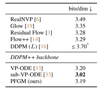
sub-VP-ODE demonstrates the best results, although its sample quality is worse than VP-ODE and PFGM. The authors leave investigations into the tradeoff between likelihood and quality to future works.
PFGM latent manipulations
Given the invertibility of M, the authors also note that samples are uniquely identified to their latent representation, allowing us to manipulate images via their latent representation. For example, simply decoding linearly interpolated points in the latent space yields a simple way to interpolate between images, demonstrated below using CelebA images:

Similarly, we can perform other manipulations such as temperature scaling, shown below again using the CelebA dataset:

Areas for improvement
PFGMs provide a very promising foundation for new avenues of research. Two such avenues are listed here.
The first avenue is a minor detail, but good for mathematical consistency. The PFGM model assumes a continuous compact distribution for mathematical convenience. While this requirement is not a problem in practice, it would be nice to prove that the results hold for non-compact distributions as well, which seems intuitively sensible given a finite integration value (which is guaranteed for probability densities).
The second area for improvement is scaling up to greater resolutions. While the authors demonstrate that PFGMs produce reasonable results at greater resolutions on 256x256 LSUN bedroom images, the ability to produce high-quality images at higher resolutions, like 512 x 512 or 1024 x 1024, has not yet been demonstrated.
One potential avenue of research would be to combine PFGMs and Diffusion Models into as components of a larger model. For example, replacing the initial base Diffusion Model in Imagen with a PFGM but leaving the Diffusion Model super-resolution chain intact could prove a powerful modification (see here for more details). As the PFGM authors note, Diffusion Models can require many function evaluations and do not provide invertibility as PFGMs do. Therefore, these weaknesses could be addressed by alternatively using a PFGM, while keeping the super-resolution chain intact to upscale the images.
Final Words
PFGMs provide a valuable contribution to the domain of generative models and early results are promising. Creative models that leverage pre-existing domain knowledge, thermodynamics and electrostatics in the cases of Diffusion Models and PFGMs respectively, provide a promising approach to the continued development of novel Machine Learning methods.
For more Machine Learning content, feel free to check out more of our blog tutorials like those on building your own text-to-image model and running Stable Diffusion.
Alternatively, check out our YouTube channel for content like our Machine Learning from Scratch series, or follow us on Twitter to stay in the loop for future content we drop.
Lorem ipsum dolor sit amet, consectetur adipiscing elit, sed do eiusmod tempor incididunt ut labore et dolore magna aliqua. Ut enim ad minim veniam, quis nostrud exercitation ullamco laboris nisi ut aliquip ex ea commodo consequat. Duis aute irure dolor in reprehenderit in voluptate velit esse cillum dolore eu fugiat nulla pariatur.